Beta Pricing

Adding a Risk-Free Asset

We know from Portfolios of Risky Assets that, with no risk-free asset available, the investment opportunity set of several risky assets is a hyperbola-shaped region bounded on the left by the minimum-variance frontier.

Adding a risk-free asset changes what is available to investors. Recall from Optimal Capital Allocation that combining the risk-free asset with a single risky portfolio P produces a straight line, the CAL of P, with intercept r_{f} and slope equal to the Sharpe ratio of P. With many risky assets to choose from, a different CAL is available for every risky portfolio P in the hyperbola-shaped opportunity set — not just for A, B, or C, but for every combination of the three.

The new investment opportunity set, once the risk-free asset is available, is the union of all these CALs. As we show below, this union is no longer the hyperbola: it is a triangle, with the best possible CAL — the one through the tangency portfolio Q — as its upper edge.

Figure 1: The figure shows the investment opportunity set generated by three risky assets A, B, and C together with their capital allocation lines. The different slopes of the CALs illustrate different Sharpe ratios for alternative risky portfolios.

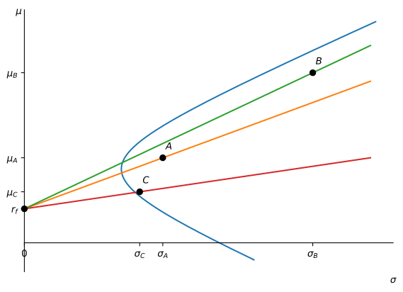
By moving the CALs higher and higher, we reach a limit on how high the Sharpe ratio of the CALs can be. Indeed, there is one portfolio Q that achieves the highest Sharpe ratio. We call this portfolio the tangency portfolio because it is, in effect, the portfolio that generates a CAL that is tangent to the original investment opportunity set generated by the three risky assets.

Figure 2: The figure shows the capital allocation line of the tangency portfolio Q obtained from the three risky assets A, B, and C.

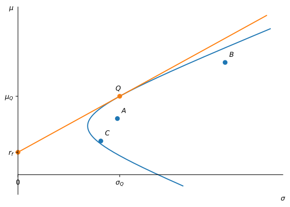
Investors that prefer portfolios with the highest Sharpe ratio will choose a portfolio located in the CAL of the tangency portfolio. We call this CAL the efficient frontier. All portfolios in this CAL are efficient since they all have the highest Sharpe ratio. Any two portfolios in this line are enough to generate all the other efficient portfolios. Any other portfolios in this economy will have lower Sharpe ratios than the tangency portfolio. To determine if a portfolio is efficient or not, just compute its Sharpe ratio and compare it to the Sharpe ratio of an efficient portfolio.

No combination of the risk-free asset with a risky portfolio can ever beat the CAL of Q, since Q has the highest possible Sharpe ratio; this line is tangent to the hyperbola exactly at Q. Going the other way — shorting Q and investing more than 100% of wealth in the risk-free asset — traces out the mirror-image line through (0, r_{f}) with the same slope in absolute value but pointing down instead of up. Unlike the CAL of Q, this line is not tangent to the hyperbola: at every risk level it lies below even the worst mean-variance inefficient combination of A, B, and C with that same volatility. This makes sense: shorting the single best portfolio to fund extra risk-free holdings is a strategy built from an efficient portfolio, so it can push further in the bad direction than any ordinary combination of A, B, and C could. Still, it is a true bound on what is achievable, so together with the CAL of Q it encloses the entire hyperbola in a triangular wedge. Once the risk-free asset is available, this triangle, not the hyperbola, is the new investment opportunity set.

Figure 3: The figure shows how the risky-asset hyperbola of A, B, and C is enclosed by two straight lines through r_{f}. The upper line is the CAL of the tangency portfolio Q and is tangent to the hyperbola. The lower line, obtained by shorting Q instead, is not tangent to the hyperbola but still bounds it from below. Once the risk-free asset is available, this triangle, not the hyperbola, is the investment opportunity set.

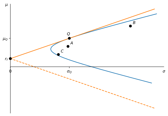
This is the real payoff of Figure 3: once the risk-free asset is available, the hyperbola itself stops mattering. Every efficient portfolio is just a combination of the risk-free asset and Q, so if an investor has mean-variance utility, their problem collapses back to the simple capital allocation problem of Optimal Capital Allocation — how much to invest in Q and how much in the risk-free asset — except that now Q is not just some risky asset, but specifically the tangency portfolio built from A, B, and C. Such an investor never needs to think about A, B, or C individually again: comparing any portfolio’s Sharpe ratio to that of Q is all that is needed.

Not every investor has mean-variance utility, so this is not a claim that everyone should hold some combination of Q and the risk-free asset — an investor with different preferences may rationally choose an inefficient portfolio. What survives regardless of preferences is pricing: as the next section shows, once Q is known to be mean-variance efficient, the expected return of every asset — whether or not it is itself efficient — is pinned down by its beta with Q and the risk-free rate. Comparing Sharpe ratios to Q’s is still the right way to check whether a portfolio is efficient, but the beta pricing relation is not something an asset can fail: it holds by construction for every asset in the economy.

Example 1 (Testing for Efficiency) You know that the tangency portfolio has an expected return of 15% with a standard deviation of returns of 20%. The risk-free rate is 5% per year. You have the following information of two risky assets.

Asset	Expected Return	Standard Deviation
A	10%	20%
B	25%	40%

Are these portfolios efficient? The Sharpe ratio of the tangency portfolio is (15 - 5) / 20 = 0.5. The Sharpe ratio of A is (10 - 5) / 20 = 0.25 < 0.5, whereas the Sharpe ratio of B is (25 - 5) / 40 = 0.5. Thus only B is an efficient portfolio.

Example 2 (Constructing an Efficient Portfolio) In Example 1, note that by investing 50% in the risk-free asset and 50% in the tangency portfolio, we obtain a portfolio with the same expected return as A but with a lower standard deviation of 0.5 \times 0.2 = 10\%.

A mean-variance investor targeting a 10% expected return would prefer this efficient portfolio to A: same expected return, less risk.

Beta Pricing

The triangle of Figure 3 describes what is attainable by combining the risk-free asset with A, B, and C. But its real usefulness goes beyond this: the tangency portfolio Q is mean-variance efficient by construction — no other portfolio has a higher Sharpe ratio — and this alone, with no reference to market equilibrium, is enough to derive a beta pricing formula for every asset or portfolio in the economy, whether or not it is one of the three risky assets used to construct Q, and whether or not it even lies inside the triangle.

Figure 4: The figure shows the tangency portfolio Q obtained from the risky assets A, B, and C. Portfolio P' is efficient and has the same expected return as P, but a lower standard deviation.

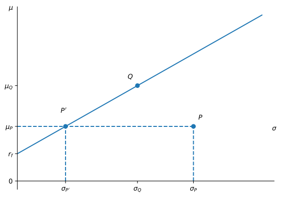
In Figure 4, portfolio P' is efficient, representing a combination of the tangency portfolio and the risk-free asset. Its return can be expressed as: r_{P'} = (1 - \beta) r_{f} + \beta r_{Q}. The residual \varepsilon = r_{P} - r_{P'} is constructed to have a mean of zero, leading to: \operatorname{E}(r_{P}) = (1 - \beta) r_{f} + \beta \operatorname{E}(r_{Q}). Additionally, the residual is orthogonal to its projection r_{P'},¹ which implies: 0 = \operatorname{Cov}(\varepsilon, r_{P'}) = \operatorname{Cov}(r_{P} - r_{P'}, r_{P'}) = \beta \operatorname{Cov}(r_{P}, r_{Q}) - \beta^{2} \operatorname{V}(r_{Q}), or equivalently: \beta = \frac{\operatorname{Cov}(r_{P}, r_{Q})}{\operatorname{V}(r_{Q})}. Nothing in this argument used market clearing, equilibrium, or any assumption about the shape of the return distribution — no normality, no symmetry, nothing beyond Q being mean-variance efficient. All that is required is that returns have well-defined (finite) means, variances, and covariances, which absence of arbitrage guarantees for any asset trading at a finite price. The same orthogonal projection argument works for any portfolio P against any efficient portfolio Q.

¹ With the risk-free asset available, let \pmb{w} hold the weights in the risky assets only, with the remainder 1 - \pmb{w}^{\top}\mathbf{1} held in the risk-free asset; the portfolio’s mean and variance are then r_{f} + \pmb{w}^{\top}(\pmb{\mu} - r_{f}\mathbf{1}) and \pmb{w}^{\top}\pmb{\Sigma}\pmb{w}, with the budget constraint already built in. Since Q is mean-variance efficient, its weights \pmb{w}_{Q} minimize variance among all portfolios with mean \mu_{Q}; the Lagrangian L(\pmb{w}, \lambda) = \pmb{w}^{\top}\pmb{\Sigma}\pmb{w} - 2\lambda\left[\pmb{w}^{\top}(\pmb{\mu} - r_{f}\mathbf{1}) - (\mu_{Q} - r_{f})\right] for this problem has first-order condition \pmb{\Sigma}\pmb{w}_{Q} = \lambda_{Q}(\pmb{\mu} - r_{f}\mathbf{1}) for some scalar \lambda_{Q} — the same condition holds for any efficient portfolio on the CAL of Q, with \lambda rescaled accordingly, except at the risk-free intercept itself, where \pmb{w} = \mathbf{0} and \lambda = 0 give a degenerate, uninformative relation. So for any portfolio i (with weights \pmb{w}_{i} in the risky assets and the remainder in the risk-free asset) \begin{aligned} \operatorname{Cov}(r_{i}, r_{Q}) &= \pmb{w}_{i}^{\top}\pmb{\Sigma}\pmb{w}_{Q} \\ &= \lambda_{Q}\pmb{w}_{i}^{\top}(\pmb{\mu} - r_{f}\mathbf{1}) = \lambda_{Q}(\mu_{i} - r_{f}), \end{aligned} an affine function of \mu_{i} alone, using \pmb{w}_{i}^{\top}(\pmb{\mu} - r_{f}\mathbf{1}) = \mu_{i} - r_{f} from the mean formula above (which holds regardless of how much of i sits in the risk-free asset). Since \varepsilon = r_{P} - r_{P'} was built so that \operatorname{E}(r_{P'}) = \operatorname{E}(r_{P}), this gives \operatorname{Cov}(r_{P}, r_{Q}) = \operatorname{Cov}(r_{P'}, r_{Q}), i.e. \operatorname{Cov}(\varepsilon, r_{Q}) = 0. Since also \operatorname{Cov}(\varepsilon, r_{f}) = 0 (as r_{f} is constant), bilinearity applied to r_{P'} = (1 - \beta) r_{f} + \beta r_{Q} gives \operatorname{Cov}(\varepsilon, r_{P'}) = 0.

Property 1 (Beta Pricing) Let Q be any mean-variance efficient portfolio. The return of any asset P can be decomposed as r_{P} = (1 - \beta_{P}) r_{f} + \beta_{P} r_{Q} + \varepsilon_{P}, where \beta_{P} = \frac{\operatorname{Cov}(r_{P}, r_{Q})}{\operatorname{V}(r_{Q})} and \operatorname{E}(\varepsilon_{P}) = \operatorname{Cov}(\varepsilon_{P}, r_{Q}) = 0. Taking expectations, \operatorname{E}(r_{P}) = (1 - \beta_{P}) r_{f} + \beta_{P} \operatorname{E}(r_{Q}).

Property 1 holds regardless of investor preferences and regardless of any assumption on the shape of the return distribution — all it needs is that returns have well-defined means, variances, and covariances. The reason is diversification, not optimization: for any asset P, the portfolio \beta_{P} r_{Q} + (1 - \beta_{P}) r_{f} matches P’s expected return while shedding \varepsilon_{P}, the piece of P’s return that is firm-specific to P and uncorrelated with Q. That piece adds variance without adding expected return, so it cannot earn a premium of its own; \operatorname{E}(r_{P}) is pinned down by \beta_{P} alone. This is a statement about pricing, not about what investors should hold. It says nothing about whether Q is anyone’s optimal portfolio, only that its efficiency is enough to price every asset relative to it.²

² In more advanced treatments, this result is restated as the pricing equation p = \operatorname{E}(mx) for a stochastic discount factor m: the mean-variance efficiency of Q is exactly what makes a linear function of r_{Q} a valid m for every asset in the economy. Existence of such an m only requires the law of one price (LOOP). Payoffs replicable at the same cost must earn the same price, which is strictly weaker than absence of arbitrage. Absence of arbitrage further requires m > 0 almost surely, and nothing here guarantees that: a mean-variance efficient Q prices every asset correctly under LOOP even if m happens to be negative in some states, in which case arbitrage opportunities can still exist.

The CAPM, covered in the next note, adds a single extra claim on top of Property 1: that the tangency portfolio Q coincides with the market portfolio M. Many textbooks blur this distinction and present the beta pricing equation as if it were a consequence of the CAPM’s equilibrium assumptions, when in fact it holds for any efficient portfolio, whether or not it is the market.

Practice Problems

These problems give you a chance to practice the concepts introduced in this chapter. Try to solve each one on your own before expanding the solution.

Problem 1 Consider an economy spanned by many risky assets and a risk-free asset that yields 5%. The tangency portfolio (Q) has an expected return of 20% and a standard deviation of 30%. Furthermore, you have information about the following funds:

Fund	Expected Return	Standard Deviation
A	15%	25%
B	8%	15%

The correlation between A and B is 0.24.

1. In a (\sigma, \mu) diagram, draw the capital allocation line (CAL) of Q, and plot funds A and B. Which portfolios are efficient? Why?
2. Peter wants to invest in an efficient portfolio (i.e. maximum Sharpe ratio) that offers an expected return of 30%. What should he do? Specify in which assets he should invest, and the standard deviation of such portfolio.
3. Christine, on the other hand, for regulatory reasons can only invest in funds A and B (and not the risk-free asset). She’s aiming for an expected return of 10%. What would you recommend to her? Please clearly indicate the composition and the standard deviation of such portfolio. Is her portfolio efficient?

Solution

1. The CAL of Q has intercept r_{f} = 5\% and slope equal to Q’s Sharpe ratio, \mathit{SR}_{Q} = \frac{\mu_{Q} - r_{f}}{\sigma_{Q}} = \frac{0.20 - 0.05}{0.30} = 0.50, so the CAL is the line \mu = 0.05 + 0.50 \, \sigma. Comparing Sharpe ratios, \mathit{SR}_{A} = \frac{0.15 - 0.05}{0.25} = 0.40, \qquad \mathit{SR}_{B} = \frac{0.08 - 0.05}{0.15} = 0.20, both fall short of \mathit{SR}_{Q} = 0.50, so A and B lie below the CAL and neither is efficient. Only portfolios on the CAL — combinations of Q with the risk-free asset — are efficient.

2. Peter should take a leveraged position in Q, borrowing at the risk-free rate to fund it. Writing w for the weight in Q, \mu_{P} = r_{f} + w (\mu_{Q} - r_{f}) \implies 0.30 = 0.05 + w \times 0.15 \implies w = 5/3 \approx 166.7\%, funded by borrowing 66.7\% of his wealth at the risk-free rate. The standard deviation of this portfolio is \sigma_{P} = w \, \sigma_{Q} = \frac{5}{3} \times 0.30 = 50\%.

3. Christine needs w_{A} \mu_{A} + (1 - w_{A}) \mu_{B} = 10\%, so w_{A} = \frac{0.10 - 0.08}{0.15 - 0.08} = 2/7 \approx 28.6\%, \qquad w_{B} = 5/7 \approx 71.4\%. The standard deviation of this portfolio is \sigma_{P} = \sqrt{w_{A}^{2} \sigma_{A}^{2} + w_{B}^{2} \sigma_{B}^{2} + 2 w_{A} w_{B} \rho_{A,B} \sigma_{A} \sigma_{B}} \approx 14.2\%. This portfolio is not efficient: an investor free to use the risk-free asset could reach the same 10\% expected return with only \sigma = (0.10 - 0.05)/0.50 = 10\% of risk, by holding 1/3 in Q and 2/3 in the risk-free asset — about four percentage points less volatility for the same expected return. Christine’s regulatory constraint against holding the risk-free asset is precisely what keeps her off the efficient frontier.

Problem 2 Consider an economy spanned by N risky assets and a risk-free asset. The tangency portfolio (Q) has an expected return of 20% and a standard deviation of 30%. You also know that Peter chooses to optimally invest in portfolio (P_{1}) with an expected return of 12% and a standard deviation of 15%.

1. Compute the risk-free rate r_{f} of this economy.
2. What is the composition of the portfolio owned by Peter?
3. Michael wants to invest optimally in a portfolio (P_{2}) that has a standard deviation of 40%. What would you recommend to him? Please clearly indicate the composition of his portfolio, and the expected return that he will be able to achieve.

Solution

1. Since Peter invests optimally, (P_{1}) is an efficient combination of Q and the risk-free asset, so Q and P_{1} lie on the same CAL. The slope of this line is \mathit{SR} = \frac{\mu_{Q} - \mu_{P_{1}}}{\sigma_{Q} - \sigma_{P_{1}}} = \frac{0.20 - 0.12}{0.30 - 0.15} = 8/15 \approx 0.533, so r_{f} = \mu_{P_{1}} - \mathit{SR} \times \sigma_{P_{1}} = 0.12 - 8/15 \times 0.15 = 4\%. As a check, 0.20 - 8/15 \times 0.30 = 4\% as well, using Q instead.

2. Writing w for the weight Peter places in Q, \mu_{P_{1}} = r_{f} + w (\mu_{Q} - r_{f}) \implies 0.12 = 0.04 + w \times 0.16 \implies w = 50\%, so Peter holds 50\% in Q and 50\% in the risk-free asset. As a check, \sigma_{P_{1}} = 0.50 \times 0.30 = 15\%, as given.

3. Michael should also combine Q with the risk-free asset, choosing the weight in Q that matches his target risk, w = \frac{\sigma_{P_{2}}}{\sigma_{Q}} = \frac{0.40}{0.30} = 4/3 \approx 133.3\%, funded by borrowing 33.3\% of his wealth at the risk-free rate. His expected return is \mu_{P_{2}} = r_{f} + w (\mu_{Q} - r_{f}) = 0.04 + \frac{4}{3} \times 0.16 \approx 25.3\%.