The Fisher Model

Introduction

The theory of finance is concerned with how investors allocate resources over time.¹ Investors must decide today how much to save, how much to consume, and how to invest their savings. Therefore, investment theory aims to determine the best way to maximize the benefit that investors derive from their consumption today and tomorrow. We denote this consumption bundle by \{C_{0}, C_{1}\}, where C_{0} is consumption today, at time 0, and C_{1} is consumption next period, at time 1. Unlike the usual consumer-theory bundle of two distinct goods, here both entries refer to the same good, consumption, just delivered at two different dates.

¹ For those interested, a more detailed explanation of the topics covered in this note can be found in Fama and Miller (1972).

Fama, E., and M. H. Miller. 1972. The Theory of Finance. Holt Rinehart & Winston.

Two distinct forces shape how investors value a consumption bundle: the passage of time, and the uncertainty surrounding future outcomes. This note isolates the role of time by assuming that C_{1} is known with certainty today; uncertainty is introduced separately in Utility Theory Under Uncertainty.

Utility Theory

We start this note by thinking about how investors can rank consumption bundles. In economics, a very convenient way to rank consumption bundles is to use a utility function. The idea of a utility function is to assign a real number to each consumption bundle since real numbers are easy to compare. A consumption bundle is then preferred to another if the utility number is larger.

For example, consider the following function,² U(C_{0}, C_{1}) = \ln(C_{0}) + \ln(C_{1}).

² Many textbooks and programming languages use \log instead of \ln. In these notes I will use \ln to denote the natural logarithm.

³ Since U(C_{0}, C_{1}) = \ln(C_{0} C_{1}), the new utility function V(C_{0}, C_{1}) = C_{0}C_{1} generates the same rankings of consumption bundles.

We can compute U(3, 2) = 1.79 and U(2.5, 2.5) = 1.83 which shows that this agent prefers consuming 2.5 units today and tomorrow over consuming three units today and two units tomorrow. For this consumer, we have that (2.5, 2.5) \succ (3, 2). The value of the utility function is irrelevant since applying any increasing function to a utility function will not change the rankings of consumption bundles.³

From the previous example, we can see that the consumer will be indifferent to some consumption bundles. For example, U(2, 1) = U(1, 2) = 0.69, which we denote by (1, 2) \sim (2, 1). The set of all consumption bundles that provide the same utility is called an indifference curve.

The figure below shows three different indifference curves. The blue line denotes all consumption bundles with a utility equal to U_{1}. The orange curve denotes all bundles that provide a utility equal to U_{2} > U_{1}. The green line provides an even higher level of utility U_{3} > U_{2}.

Figure 1: Three indifference curves over today’s consumption (C_{0}) and tomorrow’s consumption (C_{1}).

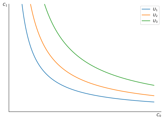
The figure also displays something that we expect to find in real life: utility should increase with consumption. In the previous example, we found that (1, 2) \sim (2, 1), but of course we would expect (1, 2) \prec (1, 3). In other words, the marginal utility of consumption must be positive for consumption in both periods, i.e., \frac{\partial U}{\partial C_{i}} > 0 for i = \{0, 1\}.

Marginal utility should also decrease with consumption, i.e., \frac{\partial^{2} U}{\partial C_{i}^{2}} < 0 for i = \{0, 1\}, since each additional unit of consumption can only increase utility at a lower rate. The first unit of consumption provides a much larger increase in utility than the last.

Example 1 In finance, it is common to use separable utility functions of the form U(C_{0}, C_{1}) = u(C_{0}) + \beta u(C_{1}), where \beta is a subjective discount factor capturing how much the investor values consumption next period relative to today. The choice u(C) = \begin{cases} \frac{C^{1 - \gamma} - 1}{1 - \gamma}, & \text{if}\ \gamma > 0, \gamma \neq 1 \\ \ln(C), & \text{if}\ \gamma = 1 \end{cases} is called power utility if \gamma \neq 1 and log utility if \gamma = 1. Log utility is in fact the limit of power utility as \gamma \rightarrow 1, since, using the approximation y^{x} = \exp(x \ln(y)) \approx 1 + x \ln(y) for small x, \lim_{\gamma \rightarrow 1} \frac{C^{1 - \gamma} - 1}{1 - \gamma} = \lim_{\gamma \rightarrow 1} \frac{1 + (1 - \gamma) \ln(C) - 1}{1 - \gamma} = \ln(C), where the middle expression uses that approximation; the error in it is of order (1-\gamma)^{2}, so it vanishes as \gamma \rightarrow 1 and the final equality is exact.

Power utility satisfies the requirements above for a well-behaved felicity function: u'(C) = C^{-\gamma} > 0 and u''(C) = -\gamma C^{-\gamma - 1} < 0, so u(C) is increasing and strictly concave. The same holds for log utility, which corresponds to the case \gamma = 1.

Figure 2 plots power utility for a few values of \gamma, including the log utility case \gamma = 1. All curves are increasing and concave, and the curvature becomes more pronounced as \gamma grows.

Figure 2: Power utility for different values of gamma.

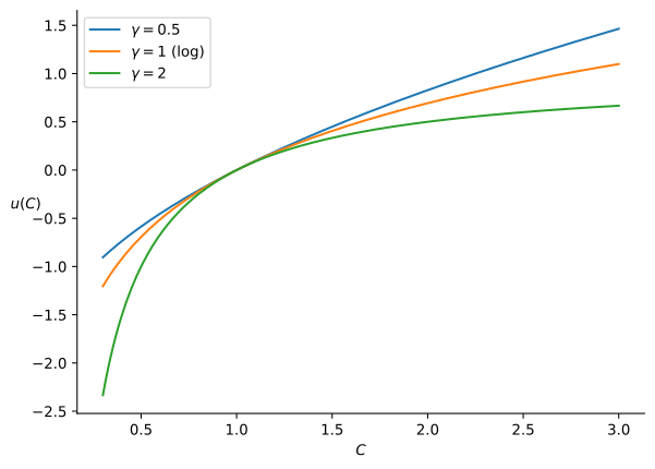
Notice in Figure 2 that u(C) dips below zero whenever C < 1, for every value of \gamma: since u(1) = 0 in all cases, u(C) < 0 for C < 1 and u(C) > 0 for C > 1. This is not a problem: as noted earlier, the level of utility carries no meaning on its own, only its ranking across bundles does. All that matters is that a higher C delivers a higher u(C), which continues to hold regardless of sign.

Example 2 Another common choice for u(C) in the separable utility function of Example 1 is u(C) = - e^{-a C}, usually called exponential utility. For a > 0, we have u'(C) = a e^{-aC} > 0 and u''(C) = -a^{2} e^{-aC} < 0, so u(C) is increasing and strictly concave.

We can compute the utility differential as dU = \frac{\partial U}{\partial C_{0}} dC_{0} + \frac{\partial U}{\partial C_{1}} dC_{1}. Since an indifference curve keeps the utility level constant, for all points in the indifference curve, we have that dU = 0, implying that \frac{dC_{1}}{dC_{0}} = - \frac{\frac{\partial U}{\partial C_{0}}}{\frac{\partial U}{\partial C_{1}}}. \tag{1} The absolute value of the derivative of C_{1} with respect to C_{0} is called the marginal rate of substitution (MRS) between C_{1} and C_{0}. The MRS compares how important it is to consume tomorrow versus today at any given point.

Production Functions

An investor must first decide how much to consume today and how much to save for the next period. Two factors determine this decision. On the one hand, the MRS determines how future consumption feels compared to current consumption. On the other hand, the ability to transform current consumption into future consumption is essential in deciding how much to consume today versus tomorrow.

We model the ability to convert current consumption into future consumption through a production function. All consumers start with a certain level of wealth, W, measured in terms of current consumption. Consumers can then decide how much to consume today, given by C_{0}^{*}, and how much to invest. An investment of K = W - C_{0}^{*} will generate C_{1}^{*} = f(K) of consumption tomorrow.

The production function combines all available investment projects and ranks them from best to worse in terms of return. Of course, if you have little to invest you want to use it in projects that have the best profitability. For example, consider the following portfolio of investment opportunities, ranked by internal rate of return (IRR).

Project	Maximum Investment	IRR
I	1	500%
II	3	300%
III	5	100%
IV	11	0%

Project I has a maximum investment of one unit of consumption and generates five additional units per unit invested. Thus, Project I transforms one unit of consumption today into six units of consumption next period. Project II transforms each additional unit of consumption today into four units of consumption tomorrow. Thus, investing four units of consumption in projects I and II generates f(4) = 1 \times 6 + 3 \times 4 = 18 units of consumption tomorrow.

Assuming that we can invest fractions of today’s consumption, we can then generate the following production function f(K).

Figure 3: The figure shows a piece-wise linear production function.

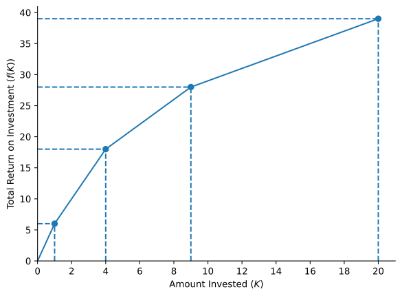
The production function we just built is continuous in its range of definition K \in [0, 20]. It is also increasing in K as long as we assume limited liability, which would be the case if you incorporate your productive activities as a firm. Note that Project IV has a net return of 0%, which means that each unit of consumption invested generates one unit of consumption tomorrow. The worst possible scenario under limited liability is that the IRR of the project is -100%. In that case all additional units invested in such a project would be destroyed, at which point the production function would be flat.

The production function in Figure 3 is also concave, which is a consequence of investing in the projects with better profitability first. Project I is the best in terms of profitability. If we only have one unit of consumption to invest we should clearly choose it. Project III will be chosen only after four units have been invested in projects I and II.

Typically, we assume that the production function is smooth such that f'(K) > 0 and f''(K) < 0, which yields a continuous, increasing, and concave function. A production function with such properties is consistent with our previous analysis.

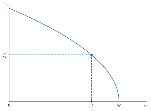
In the following, it is useful to express the function in terms of K = W - C_{0}, so that C_{1} = f(W - C_{0}). If the consumer decides to invest nothing and consume everything today, we have that K = 0 and C_{0}^{*} = W. If, on the other hand, the consumer decides to consume nothing today and invest everything, then we have that K = W and C_{0}^{*} = 0.

Figure 4: The figure shows the investment opportunity set available to an investor.

Maximizing Utility

Consider now an investor with utility function U(C_{0}, C_{1}) and initial wealth W. The investor has the ability to invest K = W - C_{0} into a production function that yields next period C_{1} = f(K). We can write the investor’s problem as follows \begin{aligned} \max_{\{C_{0}, C_{1}\}} & U(C_{0}, C_{1}) \\ \text{s.t. } & C_{1} = f(W - C_{0}) \end{aligned}

To solve the previous optimization problem, we can write the Lagrangian as \mathcal{L} = U(C_{0}, C_{1}) - \lambda (C_{1} - f(W - C_{0})).

The first-order conditions (FOC) are \begin{aligned} \frac{\partial \mathcal{L}}{\partial C_{0}} & = \frac{\partial U}{\partial C_{0}} - \lambda f'(W - C_{0}) = 0, \\ \frac{\partial \mathcal{L}}{\partial C_{1}} & = \frac{\partial U}{\partial C_{1}} - \lambda = 0, \\ \frac{\partial \mathcal{L}}{\partial \lambda} & = C_{1} - f(W - C_{0}) = 0. \end{aligned}

The first two FOCs imply that the marginal rate of substitution (MRS) must be equal to the marginal rate of transformation (MRT) between C_{1} and C_{0}. The last FOC says that whatever the investor does not consume today is invested and can be consumed tomorrow to yield C_{1} = f(W - C_{0}).

The figure below shows the optimal consumption choice. The indifference curve at the optimum is tangent to the production function, meaning that the MRS of the consumer equalizes the MRT provided by the technology.⁴

⁴ To guarantee a unique optimum, the indifference curve must be convex. Quasi-concave utility functions generate convex upper-contour sets defined as \{x \in X: U(x) \geq c \}, where X \in \mathbb{R^{N}} is the consumption set. In our case X = \mathbb{R^{2+}}. It can be shown that a function is quasi-concave if and only if U(\lambda x + (1 - \lambda) y) \geq \min(U(x), U(y)), where x, y \in X and 0 \leq \lambda \leq 1.

Figure 5: The figure shows the optimal consumption choice given a production function and initial wealth W.

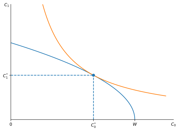
Example 3 Consider an investor with utility U(C_{0}, C_{1}) = \ln(C_{0}) + \ln(C_{1}). The investor has initial wealth W = 1 and can invest K = 1 - C_{0} in a technology that produces f(K) = \sqrt{K} next period.

The investor maximizes her utility if her consumption (C_{0}^{*}, C_{1}^{*}) satisfies \text{MRS} = \frac{C_{1}}{C_{0}} = \frac{1}{2 \sqrt{1 - C_{0}}} = \text{MRT}. Since C_{1} = \sqrt{1 - C_{0}}, we have that \frac{\sqrt{1 - C_{0}}}{C_{0}} = \frac{1}{2 \sqrt{1 - C_{0}}}, which implies that C_{0} = \frac{2}{3} and C_{1} = \sqrt{\frac{1}{3}}.

In the previous example, we have that C_{0} + C_{1} > W = 1, meaning that the production function improves the utility of the consumer compared to a simple storing technology that only allows to save consumption for later.

The Role of Capital Markets

The Production Decision

Investors can do better than autarky if they organize their economy differently. Let’s delegate the production decision to a manager with access to a technology f(K). Furthermore, assume that consumers have access to capital markets where they can borrow or lend at an interest rate r. The manager is given a certain amount of wealth W, and must decide how much to sell today, investing the rest in the technology for future production, which we denote by (Q_{0}, Q_{1}), respectively.

Shareholders expect the manager to choose (Q_{0}, Q_{1}) to maximize the value of the firm V = Q_{0} + \frac{Q_{1}}{1 + r}. The manager faces the budget constraint that he can only invest what the firm does not sell today, i.e., K = W - Q_{0}. The problem that the manager must solve is given by \max_{\{Q_{0}\}} Q_{0} + \frac{f(W - Q_{0})}{1 + r}. The FOC is \text{MRT} = f'(W - Q_{0}^{*}) = 1 + r.

The figure below shows that the optimal production choice (Q_{0}^{*}, Q_{1}^{*}) is such that at that point, the production function is tangent to the capital market line (CML) whose slope coefficient is -(1 + r).

Figure 6: The figure shows the optimal production policy for the firm given a production function and initial wealth W.

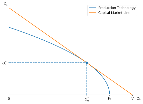
The intercept of the CML with the x-axis determines the firm value. By choosing the tangency point between the two lines, the manager maximizes the firm’s value by selecting the intercept that is furthest to the right. To increase the firm’s size, the manager would need a more significant initial investment of W.

The difference between V and W is the net present value (NPV) created using the technology. By investing an initial capital of W, shareholders now have an asset worth more than the initial investment. The manager should then accept all projects with positive NPVs.

Example 4 Consider the same production function of Example 3, i.e., f(K) = \sqrt{K} and again take W = 1. The market interest rate is r. The policy (Q_{0}^{*}, Q_{1}^{*}) that maximizes firm-value is such that \begin{aligned} \frac{1}{2 \sqrt{1 - Q_{0}^{*}}} & = 1 + r, \\ Q_{1}^{*} & = \sqrt{1 - Q_{0}^{*}}. \end{aligned} Thus, Q_{1}^{*} = \frac{1}{2 (1 + r)} and Q_{0}^{*} = 1 - \frac{1}{4 (1 + r)^2}. The value of the firm is then V = 1 - \frac{1}{4 (1 + r)^2} + \frac{1}{2 (1 + r)^{2}} = 1 + \frac{1}{4 (1 + r)^{2}}, which shows that the NPV of the technology is \frac{1}{4 (1 + r)^{2}} > 0.

Without access to capital markets, the value of the production technology is just W since this amount today can generate all possible production bundles (Q_{0}, Q_{1}). The CML is then another production function that gives investors access to superior bundles. According to the CML, the value of the technology is V > W.

The Consumption Decision

In the model, shareholders agree on how the firm should maximize its value, regardless of their utility for today’s and future consumption. An investor with initial wealth W can create the previous firm, hire a manager, and incorporate the firm. The firm will then produce Q_{0}^{*} today, invest K = W - Q_{0}^{*} and produce f(K) = Q_{1}^{*} for consumption next period.

The investor could sell the firm for V, which can be used to consume C_{0} today and invest the rest to consume C_{1} = (V - C_{0}) (1 + r) next period. The investor’s problem is \begin{aligned} \max_{\{C_{0}, C_{1}\}} & U(C_{0}, C_{1}), \\ \text{s.t. } & C_{1} = (V - C_{0}) (1 + r). \end{aligned} The Lagrangian of this problem is \mathcal{L} = U(C_{0}, C_{1}) - \lambda (C_{1} - (V - C_{0}) (1 + r)), implying the following FOC conditions \begin{aligned} \frac{\partial \mathcal{L}}{\partial C_{0}} & = \frac{\partial U}{\partial C_{0}} - \lambda (1 + r) = 0, \\ \frac{\partial \mathcal{L}}{\partial C_{1}} & = \frac{\partial U}{\partial C_{1}} - \lambda = 0, \\ \frac{\partial \mathcal{L}}{\partial \lambda} & = C_{1} - (V - C_{0}) (1 + r) = 0. \end{aligned} The first two FOCs imply that the MRS for the consumer is equal to the rate of return of the CML,i.e., \text{MRS} = \frac{\frac{\partial U}{\partial C_{0}}}{\frac{\partial U}{\partial C_{1}}} = 1 + r. The last FOC says that the present value of today’s and future consumption must equal V, i.e., V = C_{0} + \frac{C_{1}}{1 + r}.

Therefore, we have separated the decision of producing (Q_{0}^{*}, Q_{1}^{*}) given an initial wealth W, from the decision of consuming (C_{0}^{*}, C_{1}^{*}) given that the optimal production decision generates a present value of V that can be used to consume today and next period.

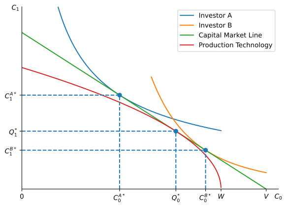
The figure below shows that the optimal consumption bundles that can be achieved by two investors with different marginal rates of substitution of consumption. Investor A prefers to give up consumption today in order to consume more next period. With access to capital markets, she now has an initial wealth of V, that allows her to save at a better marginal rate of return than with the production function alone. Investor B, on the other hand, prefers to borrow and consume more today by giving up consumption tomorrow. The existence of good functioning capital markets allows her to borrow at a cheaper rate of interest than the one provided by the production technology.

Figure 7: The figure shows the optimal production policy for the firm and optimal consumption decisions for two investors given a production function and initial wealth W.

Example 5 Consider an investor with initial wealth W who owns the technology function of Example 4. By producing Q_{0}^{*} = 1 - \frac{1}{4 (1 + r)^2} and Q_{1}^{*} = \frac{1}{2 (1 + r)}, she maximizes the firm value at V = 1 + \frac{1}{4 (1 + r)^{2}}.

Assume that the investor has a utility function of the form U(C_{0}, C_{1}) = \ln(C_{0}) + \beta \ln(C_{1}). If \beta > 1, the investor values more consumption tomorrow than today, whereas a \beta < 1 implies that the investor discounts future consumption relative to today’s consumption.

The investor must decide how much to consume today and next period given the value of her equity. At the optimum, the investor equalizes her MRS with the total return on investment so that \frac{C_{1}}{\beta C_{0}} = 1 + r. Since C_{1} = (1 + r) (V - C_{0}), we obtain C_{0}^{*} = \frac{1}{1 + \beta} V and C_{1}^{*} = (1 + r) \frac{\beta}{1 + \beta} V.

Fisher Separation Theorem

The previous analysis suggests that we can separate the firm’s investment decision, which involves deciding how much to sell today and how much to reinvest to sell tomorrow, from the investment decision faced by the consumer. This separation result is known as the Fisher Separation Theorem after economist Irving Fisher. Well-functioning capital markets play a crucial role in creating this separation.

All consumers are better off when firms maximize their values by undertaking positive NPV projects. It is the role of the firm’s manager to ensure that companies maximize their values to shareholders. Corporate finance typically studies corporate policy and firm valuation.

Given shares of these profit-maximizing firms, consumers can choose how much to invest in each firm. Investment theory explores how economic agents can optimally decide how to allocate their resources, which is what we will study in this class. We will take the investment opportunity set as given and analyze how investors can maximize their utilities.

The CML determines an equilibrium for both firms and investors. In asset pricing we typically analyze the equilibrium pricing of securities from the investors’ point of view, and it is usually called consumption-based asset pricing. The analysis in the previous section suggests that we could also study the equilibrium from the firms’ point of view, which is usually called production-based asset pricing.

Different Borrowing and Lending Rates

The Fisher separation theorem relies on the fact that capital markets allow investors to lend and borrow at the same interest rate. This assumption allows us to write that the value of consuming C_{0} today and C_{1} tomorrow is the present value of the cash flows, i.e., V = C_{0} + \frac{C_{1}}{1 + r}.

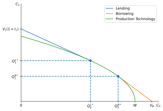
Typically, the interest rate at which investors can borrow is higher than the rate at which they can lend. In this case, the CML extends to the left with slope -(1 + r_{L}) and to the right with slope -(1 + r_{B}), where r_{L} and r_{B} denote the lending and borrowing rates, respectively.

The figure below shows the resulting investment opportunity set. At the point (Q_{0}^{L*}, Q_{1}^{L*}) the MRT is equal to 1 + r_{L}, whereas at the point (Q_{0}^{B*}, Q_{1}^{B*}) it is 1 + r_{B}.

Figure 8: The figure shows the optimal production policy for a firm when investors face different lending and borrowing rates.

There are three possibilities for the investment opportunity set:

1. An investor willing to consume C_{0} < Q_{0}^{L*} can invest V_{L} - C_{0} at r_{L} to consume C_{1} = (V_{L} - C_{0}) (1 + r_{L}) next period, where V_{L} = Q_{0}^{L*} + \frac{Q_{1}^{L*}}{1 + r_{L}}. Note that the y-intercept of this CML is V_{L} (1 + r_{L}).
2. An investor choosing to consume C_{0} such that Q_{0}^{L*} \leq C_{0} \leq Q_{0}^{B*} can consume C_{1} = f(W - C_{0}) next period, where f(\cdot) denotes the production function.
3. An investor willing to consume C_{0} > Q_{0}^{B*} can borrow C_{0} - Q_{0}^{B*} and consume C_{1} = (V_{B} - C_{0}) (1 + r_{B}) next period, where V_{B} is defined analogously.

Having different borrowing and lending rates destroys the linearity of discounting and compounding. The present value of the production technology is V_{B} whereas the future value of it is V_{L} (1 + r_{L}).

The previous analysis shows how frictions can make asset pricing problems harder to solve. In the following, we will usually assume that markets are perfect and that borrowing and lending rates are the same.

Practice Problems

These problems give you a chance to practice the concepts introduced in this chapter. Try to solve each one on your own before expanding the solution.

Conceptual Problems

Problem 1 (Ranking Consumption Bundles) An investor has utility U(C_{0}, C_{1}) = \ln(C_{0}) + \ln(C_{1}). Rank the bundles (4, 3) and (2, 5).

Solution

Since U(C_{0}, C_{1}) = \ln(C_{0} C_{1}), ranking bundles under this utility function is the same as ranking them by the product C_{0} C_{1}. We have 4 \times 3 = 12 and 2 \times 5 = 10, so U(4, 3) = \ln(12) > \ln(10) = U(2, 5), and therefore (4, 3) \succ (2, 5).

Problem 2 (Power Utility: Marginal Utility and Concavity) Consider power utility u(C) = \dfrac{C^{1 - \gamma} - 1}{1 - \gamma} with \gamma = 2. Compute u'(C) and u''(C) and evaluate them at C = 1. Verify that u(C) is increasing and strictly concave.

Solution

Differentiating, u'(C) = C^{-\gamma} = C^{-2}, \qquad u''(C) = -\gamma C^{-\gamma - 1} = -2 C^{-3}. At C = 1, u'(1) = 1 > 0 and u''(1) = -2 < 0, confirming that u(C) is increasing and strictly concave, as it must be for any \gamma > 0 and C > 0.

Problem 3 (Building a Production Function) You rank your investment opportunities by IRR as follows.

Project	Maximum Investment	IRR
I	2	300%
II	3	100%
III	5	0%

If you have K = 6 units of consumption to invest, how much consumption will you have available next period, f(6)?

Solution

Investing in the best projects first, the first 2 units go into Project I, generating 2 \times (1 + 3) = 8 units next period. The next 3 units (bringing the cumulative total invested to 5) go into Project II, generating 3 \times (1 + 1) = 6 units. The remaining 6 - 5 = 1 unit goes into Project III, generating 1 \times (1 + 0) = 1 unit. Thus, f(6) = 8 + 6 + 1 = 15.

Problem 4 (Maximizing Utility Given a Production Function) An investor has utility U(C_{0}, C_{1}) = \ln(C_{0}) + 2 \ln(C_{1}), initial wealth W = 10, and access to a production technology f(K) = \sqrt{K}. Find her optimal consumption bundle (C_{0}^{*}, C_{1}^{*}).

Solution

The investor maximizes her utility if her consumption satisfies \text{MRS} = \frac{C_{1}}{2 C_{0}} = \frac{1}{2 \sqrt{W - C_{0}}} = \text{MRT}. Since C_{1} = \sqrt{W - C_{0}}, we have that \frac{\sqrt{W - C_{0}}}{2 C_{0}} = \frac{1}{2 \sqrt{W - C_{0}}}, which implies that W - C_{0} = C_{0}, so C_{0}^{*} = W/2 = 5 and C_{1}^{*} = \sqrt{W - C_{0}^{*}} = \sqrt{5}.

Problem 5 (Optimal Production and Firm Value) A firm has access to the production technology f(K) = \sqrt{K} and initial wealth W = 1. The market interest rate is r = 50\%. Find the optimal production policy (Q_{0}^{*}, Q_{1}^{*}), the firm’s value V, and the NPV created by the technology.

Solution

Using the results of Example 4 with r = 1/2, Q_{0}^{*} = 1 - \frac{1}{4 (1 + r)^{2}} = 1 - \frac{1}{4 \times (3/2)^{2}} = 1 - \frac{1}{9} = \frac{8}{9}, \qquad Q_{1}^{*} = \frac{1}{2(1+r)} = \frac{1}{3}. The firm’s value is V = Q_{0}^{*} + \frac{Q_{1}^{*}}{1+r} = \frac{8}{9} + \frac{1/3}{3/2} = \frac{8}{9} + \frac{2}{9} = \frac{10}{9}, so the NPV created by the technology is V - W = 10/9 - 1 = 1/9.

Problem 6 (Optimal Consumption Given Firm Value) The investor in Exercise 5 owns the firm described there and has utility U(C_{0}, C_{1}) = \ln(C_{0}) + 2 \ln(C_{1}). Using the firm value V found there and r = 50\%, find her optimal consumption bundle (C_{0}^{*}, C_{1}^{*}).

Solution

From Example 5 with \beta = 2, C_{0}^{*} = \frac{1}{1+\beta} V = \frac{1}{3} \times \frac{10}{9} = \frac{10}{27}, C_{1}^{*} = (1+r) \frac{\beta}{1+\beta} V = \frac{3}{2} \times \frac{2}{3} \times \frac{10}{9} = \frac{10}{9}.

Problem 7 (Borrowing and Lending at Different Rates) A firm has production technology f(K) = \sqrt{K} and initial wealth W = 1. Investors can lend at r_{L} = 50\% but must borrow at r_{B} = 100\%. Find the tangency points (Q_{0}^{L*}, Q_{1}^{L*}) and (Q_{0}^{B*}, Q_{1}^{B*}) on the production frontier, and describe what happens to an investor who wants to consume between these two points today.

Solution

Applying the tangency condition f'(W - Q_{0}) = 1 + r at each rate, Q_{0}^{L*} = 1 - \frac{1}{4(1+r_{L})^{2}} = 1 - \frac{1}{9} = \frac{8}{9}, \qquad Q_{1}^{L*} = \frac{1}{2(1+r_{L})} = \frac{1}{3}, Q_{0}^{B*} = 1 - \frac{1}{4(1+r_{B})^{2}} = 1 - \frac{1}{16} = \frac{15}{16}, \qquad Q_{1}^{B*} = \frac{1}{2(1+r_{B})} = \frac{1}{4}. An investor choosing to consume C_{0} between Q_{0}^{L*} = 8/9 and Q_{0}^{B*} = 15/16 neither borrows nor lends: she simply consumes C_{1} = f(W - C_{0}) directly from the technology, since at those intermediate levels neither the lending nor the borrowing rate is attractive enough to justify trading away from the production frontier.

Comprehensive Problems

Problem 8 (Portfolio Choice With and Without Capital Markets) Suppose an investor’s production opportunity set in a world with perfect certainty consists of the following investment projects:

Project	Maximum Investment	IRR
A	$1,000,000	8%
B	$1,000,000	25%
C	$2,000,000	4%
D	$3,000,000	40%

Consider an investor with utility function U(C_{0}, C_{1}) = C_{0} + 0.9 C_{1}. This investor has $7,000,000 in wealth.

1. If the investor has no access to capital markets.
   1. What is the value of her portfolio of projects, measured in today’s consumption?
   2. How much should she consume today and how much next period?
2. Suppose now that a new bank comes to town, that allows the investor to borrow or lend at the interest rate of 10% per period.
   1. What is the value of her portfolio of projects?
   2. How much should she consume today and how much next period?
3. If the bank was forced to close right after opening, before the investor could act on it, how much would the government have to pay her to leave her as well off as she would have been with permanent access to the bank?

Solution

Since U(C_{0}, C_{1}) = C_{0} + 0.9 C_{1} is linear, indifference curves are straight lines with constant MRS = 1/0.9 = 1.1111, i.e., the investor requires a return of at least 1/0.9 - 1 \approx 11.11\% to give up consumption today. Ranking the projects by IRR gives D (40\%) > B (25\%) > A (8\%) > C (4\%).

a. Without access to capital markets. The investor can only transform C_{0} into C_{1} through the projects themselves, so with linear utility each project should be either fully funded or left untouched, and only projects whose IRR exceeds her required return of 11.11\% are worth funding. This means funding D and B in full, since A (8\%) and C (4\%) both fall short of 11.11\%.

1. Since U has a unit coefficient on C_{0}, U(C_{0}, C_{1}) = C_{0} + 0.9 C_{1} is itself denominated in today’s dollars and gives the value of any consumption bundle. Investing $3,000,000 in D and $1,000,000 in B leaves C_{0} = 7{,}000{,}000 - 4{,}000{,}000 = \$3{,}000{,}000 uninvested and generates C_{1} = 3{,}000{,}000 \times 1.40 + 1{,}000{,}000 \times 1.25 = \$5{,}450{,}000 next period. The value of her portfolio is therefore U^{a} = 3{,}000{,}000 + 0.9 \times 5{,}450{,}000 = \$7{,}905{,}000.
2. She should consume C_{0}^{*} = \$3{,}000{,}000 today and C_{1}^{*} = \$5{,}450{,}000 next period.

b. With access to capital markets at r = 10\%. The production and consumption decisions now separate, and the firm should fund every project whose IRR exceeds the market rate of 10\%. Since A’s IRR of 8\% still falls short of 10\%, the optimal production decision is unchanged: fund D and B only, so Q_{0}^{*} = \$3{,}000{,}000 and Q_{1}^{*} = \$5{,}450{,}000.

1. The value of the portfolio is now its present value at the market rate, V = 3{,}000{,}000 + \frac{5{,}450{,}000}{1.10} = \$7{,}954{,}545.45.
2. Substituting the budget constraint C_{1} = (V - C_{0})(1+r) into U gives U = C_{0} + 0.9 (1.10) (V - C_{0}) = 0.99 V + 0.01 C_{0}. Since the coefficient on C_{0} is positive, utility is increasing in C_{0}, so the investor should consume as much as possible today: C_{0}^{*} = V = \$7{,}954{,}545.45 and C_{1}^{*} = 0. Intuitively, the market only compensates 10\% for delaying consumption, below the 11.11\% she requires, so she prefers to cash out the entire value of the firm today rather than lend any of it.

c. Compensation for closing the bank. Because U is a money-metric utility (unit coefficient on C_{0}), the compensation the government must pay equals the difference in the value of her portfolio with and without access to the bank, V - U^{a} = 7{,}954{,}545.45 - 7{,}905{,}000 = \$49{,}545.45.

Problem 9 (Optimal Consumption, Present Value, and NPV of a Technology) Consider an investor with utility U(C_{0}, C_{1}) = \ln(C_{0}) + 2 \ln(C_{1}) for consumption today and next period. The investor has initial wealth W = 1 and can invest K = 1 - C_{0} in a technology that produces f(K) = \sqrt{K} next period.

1. Compute the optimal consumption at dates 0 and 1.

Assume now that the investor has access to capital markets and can borrow or lend at r.

2. Compute the present value and the net present value of the technology.
3. If the investor sells the company at the value computed in b., what is her optimal consumption now?

Solution

a. Optimal consumption without capital markets. As in Example 3, the investor maximizes utility where MRS equals MRT: \text{MRS} = \frac{C_{1}}{2 C_{0}} = \frac{1}{2 \sqrt{1 - C_{0}}} = \text{MRT}. Since C_{1} = \sqrt{1 - C_{0}}, \frac{\sqrt{1 - C_{0}}}{2 C_{0}} = \frac{1}{2 \sqrt{1 - C_{0}}} \implies 1 - C_{0} = C_{0} \implies C_{0}^{*} = \frac{1}{2}, so C_{1}^{*} = \sqrt{1 - 1/2} = 1/\sqrt{2} \approx 0.7071.

b. Present value and NPV. As in Example 4 with W = 1, the firm maximizes its value where f'(W - Q_{0}) = 1 + r, giving Q_{0}^{*} = 1 - \frac{1}{4(1+r)^{2}}, \qquad Q_{1}^{*} = \frac{1}{2(1+r)}. The present value of the technology is V = Q_{0}^{*} + \frac{Q_{1}^{*}}{1+r} = 1 + \frac{1}{4(1+r)^{2}}, so the net present value is \text{NPV} = V - W = \dfrac{1}{4(1+r)^{2}}.

c. Optimal consumption after selling the firm. As in Example 5 with \beta = 2, C_{0}^{*} = \frac{1}{1+\beta} V = \frac{V}{3} = \frac{1}{3} \left(1 + \frac{1}{4(1+r)^{2}}\right), C_{1}^{*} = (1+r) \frac{\beta}{1+\beta} V = \frac{2(1+r)}{3} \left(1 + \frac{1}{4(1+r)^{2}}\right) = \frac{2(1+r)}{3} + \frac{1}{6(1+r)}.