Probability Basics
This note introduces the concepts used to model uncertainty: outcomes and events, a probability measure that assigns each outcome a number representing its probability, and random variables that assign payoffs to outcomes. From these we define the expectation, variance, and covariance of a random variable, the tools used throughout the course to measure the return and risk of a portfolio.
In the following, there is only a finite number of future possibilities to simplify the mathematical exposition. For example, the future price of a stock can go up, stay constant, or go down. However, all the results presented in this chapter hold if we relax this assumption and allow for an infinite number of future outcomes.
We start by reviewing basic set theory, since sets are the natural language for describing a collection of possible future outcomes. From there, we build up the notions of events, random variables, and probability, and use them to define the expectation, variance, and covariance of asset payoffs, which are the building blocks for reasoning about risk and diversification in a portfolio.
Sets
A set is a collection of objects. The objects of a set can be anything you want. For example, a set may contain numbers, letters, cars, or pictures. In our case, we will be concerned with sets that contain future possibilities or outcomes that can occur.
One way to define a set is to enumerate its elements. For example, the set of all integers from 1 to 10 is A = \{1, 2, 3, 4, 5, 6, 7, 8, 9, 10\}. Once we have defined a set, we can determine whether an object is an element of the set or not. For example, the number 3 is an element of A whereas the number 20 is not. We use the symbol \in to denote membership of a set and \notin to denote the contrary. Therefore, we have that 3 \in A and 20 \notin A.
Some sets can have an infinite number of elements. For example, the natural numbers are defined as \mathbb{N} = \{0, 1, 2, 3, \ldots\}, where the triple dots mean that if n is in \mathbb{N}, then n+1 is also in \mathbb{N}.
Since all elements of A are also members of \mathbb{N}, we say that A is a subset of \mathbb{N} and write it as A \subset \mathbb{N}. Using this terminology, we can redefine the set A defined above in a more Pythonic way: A = \{ n \in \mathbb{N} : n < 11 \}. If we are studying sets of natural numbers, it makes sense to define the universe to be \mathbb{N} and sets under study will be subsets of the universe.
Now, define the set B as B = \{6, 7, 8, 9, 10, 11, 12, 13, 14, 15\}.
The intersection between A and B is the set denoted A \cap B whose members are both in A and B. Using the sets defined above, we have that A \cap B = \{6, 7, 8, 9, 10\}. The union of the sets A and B is the set denoted A \cup B whose members are either in A, B, or both. Thus, using our previously defined sets we have that A \cup B = \{1, 2, 3, \ldots , 14, 15\}. The set difference of A and B is the set denoted A \setminus B whose members are in A but are not members of B. Thus, A \setminus B = \{1, 2, 3, 4, 5\} and B \setminus A = \{11, 12, 13, 14, 15\}. The complement of A is the set denoted by A^{C} whose members are not in A. Of course this statement only makes sense if we define a universe where the elements not in A can live. If the universe is \mathbb{N}, then A^{C} = \mathbb{N} \setminus A = \{11, 12, 13, \ldots\}. Similarly, B^{C} = \{0, 1, 2, 3, 4, 5\} \cup \{16, 17, 18, \ldots\}. Note that if you take all the elements of A out of A you end up with an empty set, that is A \setminus A = \{\}. We typically denote the empty set by \emptyset, but is good to keep in mind that \emptyset = \{\}. In our universe of natural numbers, no natural number is a member of the empty set. We can write this formally as n \notin \emptyset, \forall n \in \mathbb{N}. Thus, the empty set is a subset of any subset of \mathbb{N}.
The cardinality of the set A, denoted by |A|, counts the number of elements in A. We then have that |A| = |B| = 10. The empty set has cardinality 0 whereas the cardinality of \mathbb{N} is denoted \aleph_{0}.
The power set of a set C, denoted by \mathcal{P}(C), is the set containing all possible subsets of C. For example, if C = \{1, 2, 3\}, then |C| = 3 and \mathcal{P}(C) = \{\{\}, \{1\}, \{2\}, \{3\}, \{1, 2\}, \{2, 3\}, \{1, 3\}, \{1, 2, 3\}\}. Clearly, the power sets of A and B are much bigger. For a given set A, the cardinality of its power set is 2^{|A|}. Therefore, \mathcal{P}(A) and \mathcal{P}(B) each contain 2^{10} = 1024 different sets.
Finally, the Cartesian product of A and B is the set denoted by A \times B whose members are all the pairwise combinations of the elements of A and B. \begin{array}{c|cccc} A \times B & 6 & 7 & \dots & 15 \\ \hline 1 & (1, 6) & (1, 7) & \dots & (1, 15) \\ 2 & (2, 6) & (2, 7) & \dots & (2, 15) \\ \vdots & \vdots & \vdots & \ddots & \vdots \\ 10 & (10, 6) & (10, 7) & \dots & (10, 15) \end{array}
The cardinality of A \times B is equal to the product of the cardinalities of A and B, i.e., |A \times B| = |A| \times |B|.
Outcomes and Events
In probability theory, a finite sample space is a non-empty finite set denoted by \Omega. The sample space includes all possible outcomes that can occur. A probability measure is a function that assigns to each element \omega of \Omega a number in [0, 1] so that \sum_{\omega \in \Omega} \operatorname{P}(\omega) = 1. An event A is a subset of \Omega, and we define the probability of that event occurring as \operatorname{P}(A) = \sum_{\omega \in A} \operatorname{P}(\omega). \tag{1} Such a finite probability space is denoted by (\Omega, \operatorname{P}).
An immediate consequence of (1) is that \operatorname{P}(\Omega) = 1. Furthermore, if A and B are disjoint sets of \Omega we have that \begin{aligned} \operatorname{P}(A \cup B) & = \sum_{\omega \in A \cup B} \operatorname{P}(\omega) \\ & = \sum_{\omega \in A} \operatorname{P}(\omega) + \sum_{\omega \in B} \operatorname{P}(\omega) \\ & = \operatorname{P}(A) + \operatorname{P}(B). \end{aligned} If we denote by A^{C} the complement of A in \Omega, the last expression implies that \operatorname{P}(A) + \operatorname{P}(A^{C}) = 1. Also, because \Omega^{C} = \emptyset, we also have that \operatorname{P}(\Omega) + \operatorname{P}(\emptyset) = 1, or \operatorname{P}(\emptyset) = 0.
Example 1 If \Omega = \{ \omega_{1}, \omega_{2}, \omega_{3} \}, then \begin{aligned} \mathcal{P}(\Omega) & = \{ \emptyset, \{\omega_{1}\}, \{\omega_{2}\}, \{\omega_{3}\}, \{\omega_{1}, \omega_{2}\}, \{\omega_{2}, \omega_{3}\}, \{\omega_{1}, \omega_{3}\}, \{\omega_{1}, \omega_{2}, \omega_{3}\}\} \end{aligned} defines the collection of all possible events that we can measure. As we saw previously, the cardinality of \mathcal{P}(\Omega) grows exponentially with the size of \Omega.
The function \operatorname{P} such that \operatorname{P}(\omega_{1}) = 1/2, \operatorname{P}(\omega_{2}) = 1/4, and \operatorname{P}(\omega_{3}) = 1/4 defines a probability measure on \Omega. For example, we have that \operatorname{P}(\{\omega_{1}, \omega_{3}\}) = 1/2 + 1/4 = 3/4.
Random Variables
Definition
Sets and events tell us what can happen, but investment theory is ultimately about numbers: a stock’s return, a portfolio’s payoff, next quarter’s dividend. A random variable is the tool that attaches a number to each possible outcome, which is exactly what we need to talk about returns instead of abstract states of the world.
If (\Omega, \operatorname{P}) is a finite probability space, a random variable is a real-valued function defined on \Omega.
Example 2 Consider a sample space with four possible outcomes \Omega = \{ \omega_{1}, \omega_{2}, \omega_{3}, \omega_{4} \}. The table below describes the possible values of three random variables denoted by X, Y and Z.
| Outcome | X | Y | Z |
|---|---|---|---|
| \omega_{1} | -10 | 20 | 15 |
| \omega_{2} | -5 | 10 | -10 |
| \omega_{3} | 5 | 0 | 15 |
| \omega_{4} | 10 | 0 | -10 |
Observing the values of X provides perfect information about which event happened. For example, if X = 5 then we know that \omega_{3} occurred.
Knowing the values of Y or Z, on the other hand, does not provide the same amount of information. If we learn that Y = 0 we only know that either \omega_{3} or \omega_{4} occurred. If we denote by \mathcal{F}_{Y} the set of events that can be generated by Y, we have that \mathcal{F}_{Y} = \{ \emptyset, \{\omega_{1}\}, \{\omega_{2}\}, \{\omega_{1}, \omega_{2}\}, \{\omega_{3}, \omega_{4}\}, \{\omega_{1}, \omega_{3}, \omega_{4}\}, \{\omega_{2}, \omega_{3}, \omega_{4}\}, \Omega\}. The information set provided by Z is even smaller, since \mathcal{F}_{Z} = \{ \emptyset, \{\omega_{1}, \omega_{3}\}, \{\omega_{2}, \omega_{4}\}, \Omega\}. Thus, a random variable does not necessarily provide all the information generated by the probability space \Omega.
Expectation and Variance
If X is a random variable defined on a finite probability space (\Omega, \operatorname{P}), the expectation or expected value of X is defined to be \operatorname{E}(X) = \sum_{\omega \in \Omega} X(\omega) \operatorname{P}(\omega), whereas the variance of X is \operatorname{V}(X) = \operatorname{E}(X - \operatorname{E}(X))^{2}. The standard deviation is the square-root of the variance, i.e., \sigma_{X} = \sqrt{\operatorname{V}(X)}.
Example 3 Consider the sample space \Omega = \{ \omega_{1}, \omega_{2}, \omega_{3} \} in which we define the probability measure \operatorname{P} such that \operatorname{P}(\omega_{1}) = 1/2, \operatorname{P}(\omega_{2}) = 1/4, and \operatorname{P}(\omega_{3}) = 1/4. There are two random variables X and Y that take values in \Omega according to the table below.
| Outcome | Probability | X | Y |
|---|---|---|---|
| \omega_{1} | 1/2 | 10 | 2 |
| \omega_{2} | 1/4 | 8 | 40 |
| \omega_{3} | 1/4 | 4 | 20 |
Using this information, we can compute the expectation of each random variable.
\begin{aligned} \operatorname{E}(X) & = \frac{1}{2} \times 10 + \frac{1}{4} \times 8 + \frac{1}{4} \times 4 = 8, \\ \operatorname{E}(Y) & = \frac{1}{2} \times 2 + \frac{1}{4} \times 40 + \frac{1}{4} \times 20 = 16. \end{aligned} Having computed the expectations of X and Y, we can compute their variances as \begin{aligned} \operatorname{V}(X) & = \frac{1}{2} \times (10 - 8)^{2} + \frac{1}{4} \times (8 - 8)^{2} + \frac{1}{4} \times (4 - 8)^{2} = 6, \\ \operatorname{V}(Y) & = \frac{1}{2} \times (2 - 16)^{2} + \frac{1}{4} \times (40 - 16)^2 + \frac{1}{4} \times (20 - 16)^2 = 246. \end{aligned} Finally, the standard deviations of X and Y are \sigma_{X} = \sqrt{6} \approx 2.45 and \sigma_{Y} = \sqrt{246} \approx 15.68, respectively.
Covariance
The covariance between two random variables X and Y defined on a probability space (\Omega, \operatorname{P}) is defined as \operatorname{Cov}(X, Y) = \operatorname{E}(X - \operatorname{E}(X)) (Y - \operatorname{E}(Y)), and their correlation is \rho_{X, Y} = \frac{\operatorname{Cov}(X, Y)}{\sigma_{X} \sigma_{Y}}. The correlation between any two random variables is always between -1 and 1.1
1 Define the standardized random variables U = \dfrac{X - \operatorname{E}(X)}{\sigma_{X}} and V = \dfrac{Y - \operatorname{E}(Y)}{\sigma_{Y}}, so that \operatorname{E}(U^{2}) = \operatorname{E}(V^{2}) = 1 and \operatorname{E}(UV) = \rho_{X,Y}. We can then compute 0 \leq \operatorname{E}(U - V)^{2} = 2 - 2 \rho_{X,Y}, which implies \rho_{X,Y} \leq 1. Similarly, 0 \leq \operatorname{E}(U + V)^{2} = 2 + 2 \rho_{X,Y}, which implies \rho_{X,Y} \geq -1. Thus, we conclude that -1 \leq \rho_{X,Y} \leq 1.
Example 4 Continuing with Example 3, we have that \operatorname{Cov}(X, Y) = \frac{1}{2} \times (10 - 8)(2 - 16) + \frac{1}{4} (8 - 8)(40 - 16) + \frac{1}{4} (4 - 8)(20 - 16) = -18. Thus, \rho_{X, Y} \approx -0.47.
The covariance of X and Y can also be expressed as2 \operatorname{Cov}(X, Y) = \operatorname{E}(X Y) - \operatorname{E}(X) \operatorname{E}(Y).
2 From the definition of covariance and the linearity of expectation we have that \begin{aligned} \operatorname{Cov}& (X, Y) \\ & = \operatorname{E}(X - \operatorname{E}(X))(Y - \operatorname{E}(Y)) \\ & = \operatorname{E}[X (Y - \operatorname{E}(Y))] - \operatorname{E}[\operatorname{E}(X) (Y - \operatorname{E}(Y))] \\ & = \operatorname{E}(XY) - \operatorname{E}[X \operatorname{E}(Y)] - \operatorname{E}(X) \operatorname{E}(Y - \operatorname{E}(Y)) \\ & = \operatorname{E}(XY) - \operatorname{E}(X) \operatorname{E}(Y). \\ \end{aligned}
Probability Mass Function
For discrete random variables, the probability mass function (or pmf) is a real-valued function that specifies the probability that the random variable X is equal to a certain value x, i.e., p_{X}(x) = \operatorname{P}(\omega \in \Omega : X(\omega) = x).
Example 5 Suppose we define a probability measure \operatorname{P} to the random variables X and Y defined in Example 2 according to the table below.
| Outcome | \operatorname{P} | X | Y |
|---|---|---|---|
| \omega_{1} | 0.10 | -10 | 20 |
| \omega_{2} | 0.30 | -5 | 10 |
| \omega_{3} | 0.40 | 5 | 0 |
| \omega_{4} | 0.20 | 10 | 0 |
We have that the probability mass function of X is p_{X}(x) = \begin{cases} 0.10 & \text{if } x = -10, \\ 0.30 & \text{if } x = -5, \\ 0.40 & \text{if } x = 5, \\ 0.20 & \text{if } x = 10. \end{cases}
The probability mass function of Y takes only three different values for Y. p_{Y}(y) = \begin{cases} 0.60 & \text{if } y = 0, \\ 0.30 & \text{if } y = 10, \\ 0.10 & \text{if } y = 20. \end{cases}
It is sometimes easier to visualize the probability mass function by plotting the probability of different values of the random variable.
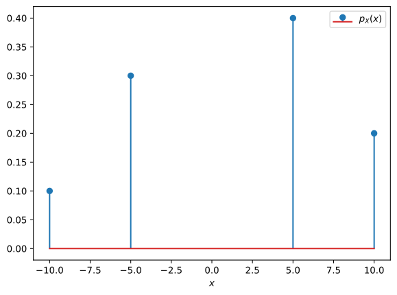
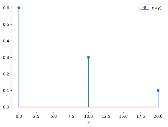
It is apparent from the pictures that p_{X}(x) = 0 if x \notin \{-10, -5, 5, 10\}. Indeed, the set \{\omega \in \Omega : X(\omega) = x \} is empty for all x not equal to -10, -5, 5, or 10. Similarly, p_{Y}(y) = 0 if y \notin \{0, 10, 20\}.
To simplify notation, we will often write \{X = x\} to denote the set \{\omega \in \Omega : X(\omega) = x\}. Using this notation, we have that p_{X}(x) = \operatorname{P}(X = x).
The support of X is the set R_{X} = \{x \in \mathbb{R} : p_{X}(x) > 0\}, that is, the values X can actually take with positive probability. Since \Omega is finite, R_{X} is finite as well, say R_{X} = \{x_{1}, x_{2}, \ldots, x_{m}\}. Using this notation we can re-write the expectation of X as \operatorname{E}(X) = \sum_{x \in R_{X}} x\, p_{X}(x) = \sum_{i = 1}^{m} x_{i} p_X(x_{i}), \tag{2} which is commonly used in statistics. Similarly, the variance of X becomes \operatorname{V}(X) = \sum_{x \in R_{X}} (x - \operatorname{E}(X))^{2}\, p_{X}(x).
For two random variables X and Y defined in (\Omega, \operatorname{P}), the set \{X = x, Y = y\} denotes all outcomes in \Omega that satisfy \{X = x\} and \{Y = y\}. Therefore, we have that \{X = x, Y = y\} = \{X = x\} \cap \{Y = y\}. The function p_{X, Y}(x, y) = \operatorname{P}(X = x, Y = y) is called the joint probability mass function of X and Y. Similarly to R_{X}, the support of Y is R_{Y} = \{y \in \mathbb{R} : p_{Y}(y) > 0\}, which we write as R_{Y} = \{y_{1}, y_{2}, \ldots, y_{n}\}.
Example 6 The joint pmf of the random variables defined in Example 5 is given in the table below.
\begin{array}{c|cccc} X \setminus Y & 0 & 10 & 20 \\ \hline -10 & 0 & 0 & 0.1 \\ -5 & 0 & 0.3 & 0 \\ 5 & 0.4 & 0 & 0 \\ 10 & 0.2 & 0 & 0 \end{array} The function p_{X, Y}(x, y) has many zeros since in Example 5 there are only four outcomes. Any other outcome then has probability zero of occurring.
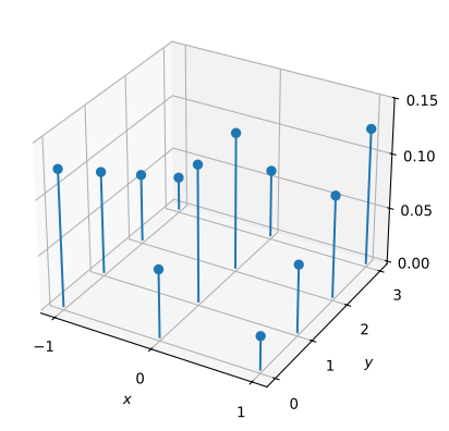
Example 7 We can generate any joint pmf for two random variables as long as the sum of all probabilities is equal to one. The table below reports the joint probabilities of a random variable X taking values in [-1, 0, 1] and a random variable Y taking values in [0, 1, 2, 3]. \begin{array}{c|cccc} X \setminus Y & 0 & 1 & 2 & 3 \\ \hline -1 & 0.12500 & 0.09375 & 0.06250 & 0.03125 \\ 0 & 0.06250 & 0.12500 & 0.12500 & 0.06250 \\ 1 & 0.03125 & 0.06250 & 0.09375 & 0.12500 \end{array}
In this case the underlying probability space has at least 3 \times 4 = 12 possible outcomes. The figure below plots the joint pmf of X and Y.
To plot the joint pmf of two random variables we need a three-dimensional graph.
We can use the joint pmf to compute the expectation of a function of two random variables. Indeed, we have that \operatorname{E}(f(X, Y)) = \sum_{i = 1}^{m} \sum_{j = 1}^{n} f(x_{i}, y_{j}) p_{X, Y}(x_{i}, y_{j}). \tag{3} If we write \mu_{X} = \operatorname{E}(X) and \mu_{Y} = \operatorname{E}(Y), equation (3) implies that the covariance of X and Y can be computed as \operatorname{Cov}(X, Y) = \sum_{i = 1}^{m} \sum_{j = 1}^{n} (x_{i} - \mu_{X})(y_{j} - \mu_{Y}) p_{X, Y}(x_{i}, y_{j}). The joint pmf contains all the information of X and Y since we can recover the individual pmfs of X and Y from it. Indeed, we have that p_{X}(x) = \sum_{j = 1}^{n} p_{X, Y}(x, y_{j}) and p_{Y}(y) = \sum_{i = 1}^{m} p_{X, Y}(x_{i}, y). It is important to note that the joint pmf not only contains the individual information of two random variables but also captures their mutual dependence.
Independence
Independence formalizes the idea that learning about one random variable tells you nothing about another. As we will see in this section, independence is a notion that is stronger than zero covariance between two random variables.
We say that two events A and B are independent if \operatorname{P}(A \cap B) = \operatorname{P}(A) \operatorname{P}(B).
Example 8 Suppose that the weather tomorrow can be either sunny, fair or rainy. In addition, a certain stock tomorrow can either go up or down in price.
We can define W = \{\text{sunny}, \text{fair}, \text{rainy}\} and S = \{\text{up}, \text{down}\}. The set of outcomes can be described as all possible pairwise combinations of weather tomorrow and the stock price movement. The sample space \Omega is then the cartesian product of W and S, i.e., \Omega = W \times S.
We can then define the weather events \begin{aligned} \text{Sunny} & = \{(\text{sunny}, \text{up}), (\text{sunny}, \text{down})\}, \\ \text{Fair} & = \{(\text{fair}, \text{up}), (\text{fair}, \text{down})\}, \\ \text{Rainy} & = \{(\text{rainy}, \text{up}), (\text{rainy}, \text{down})\}. \end{aligned}
The table below describes the probabilities for tomorrow’s weather.
| Weather | Sunny | Fair | Rainy |
|---|---|---|---|
| Probability | 0.3 | 0.5 | 0.2 |
Similarly, the stock events can be defined as \begin{aligned} \text{Up} & = \{(\text{sunny}, \text{up}), (\text{fair}, \text{up}), (\text{rainy}, \text{up})\}, \\ \text{Down} & = \{(\text{sunny}, \text{down}), (\text{fair}, \text{down}), (\text{rainy}, \text{down})\}. \\ \end{aligned}
The probabilities of the stock price going up or down are described in the table below.
| Stock | Up | Down |
|---|---|---|
| Probability | 0.6 | 0.4 |
If the weather does not affect the likelihood of the stock going up or down, we should expect to see on sunny days 60% of the time the stock going up and 40% of those days the stock going down.
That is, if the weather tomorrow and the stock price movement are independent events, we should expect \operatorname{P}(\text{Stock} \cap \text{Weather}) = \operatorname{P}(\text{Stock}) \operatorname{P}(\text{Weather}), where \text{Stock} is either \text{Up} or \text{Down}, and \text{Weather} is either \text{Sunny}, \text{Fair}, or \text{Rainy}.
The table below describes the combined probabilities of the stock price movement and the weather tomorrow that are consistent with the independence of those events.
| Stock\Weather | Sunny | Fair | Rain |
|---|---|---|---|
| Up | 0.18 | 0.30 | 0.12 |
| Down | 0.12 | 0.20 | 0.08 |
In the table, the weather does not change the relative proportions of the probabilities for the stock price.
The previous example shows how to generate independent events out of two finite probability spaces (\Omega_{1}, \operatorname{P}_{1}) and (\Omega_{2}, \operatorname{P}_{2}). If we define \Omega = \Omega_{1} \times \Omega_{2} and let \operatorname{P}(\omega_{1}, \omega_{2}) = \operatorname{P}_{1}(\omega_{1}) \operatorname{P}_{2}(\omega_{2}) for each \omega_{1} \in \Omega_{1} and \omega_{2} \in \Omega_{2}, the pair (\Omega, \operatorname{P}) is a well-defined finite probability space. In this new probability space, the events A = \{\omega_{1}\} \times \Omega_{2} and B = \Omega_{1} \times \{\omega_{2}\} are independent for any \omega_{1} \in \Omega_{1} and \omega_{2} \in \Omega_{2}.3
3 To prove this statement, we need to show that \operatorname{P}(A \cap B) = \operatorname{P}(A) \operatorname{P}(B). Indeed, we have that \begin{aligned} \operatorname{P}(A) & = \sum_{\omega_{2} \in \Omega_{2}} \operatorname{P}(\omega_{1}, \omega_{2}) \\ & = \sum_{\omega_{2} \in \Omega_{2}} \operatorname{P}_{1}(\omega_{1}) \operatorname{P}_{2}(\omega_{2}) \\ & = \operatorname{P}_{1}(\omega_{1}) \sum_{\omega_{2} \in \Omega_{2}} \operatorname{P}_{2}(\omega_{2}) \\ & = \operatorname{P}_{1}(\omega_{1}). \end{aligned} Similarly, \operatorname{P}(B) = \operatorname{P}_{2}(\omega_{2}). Since A \cap B = \{(\omega_{1}, \omega_{2})\}, we have that \operatorname{P}(A \cap B) = \operatorname{P}(A) \operatorname{P}(B), proving that A and B are independent.
Example 9 The sample space \Omega is always independent from any event A \subset \Omega since \operatorname{P}(A \cap \Omega) = \operatorname{P}(A) = \operatorname{P}(A) \operatorname{P}(\Omega). Intuitively, an outcome always happens independently of whether A happens or not.
Two random variables X and Y are independent if the events \{X = x\} and \{Y = y\} are independent. Thus, if X and Y are independent we have that \operatorname{P}(X = x, Y = y) = \operatorname{P}(X = x) \operatorname{P}(Y = y), or equivalently p_{X, Y}(x, y) = p_{X}(x) p_{Y}(y).
An important consequence of independence is that if X and Y are two independent random variables, then4 \operatorname{E}(XY) = \operatorname{E}(X) \operatorname{E}(Y). \tag{4}
4 If the domains of X and Y are \{x_{1}, x_{2}, \ldots, x_{m}\} and \{y_{1}, y_{2}, \ldots, y_{n}\}, respectively, we can then write \begin{aligned} \operatorname{E}(X) & = \sum_{i = 1}^{m} x_{i} p_{X}(x_{i}), \\ \operatorname{E}(Y) & = \sum_{j = 1}^{n} y_{j} p_{Y}(y_{j}). \end{aligned} Thus, \begin{aligned} \operatorname{E}(X) \operatorname{E}(Y) & = \left( \sum_{i = 1}^{m} x_{i} p_{X}(x_{i}) \right) \left( \sum_{j = 1}^{n} y_{j} p_{Y}(y_{j}) \right) \\ & = \sum_{i = 1}^{m} \sum_{j = 1}^{n} x_{i} y_{j} p_{X}(x_{i}) p_{Y}(y_{j}) \\ & = \sum_{i = 1}^{m} \sum_{j = 1}^{n} x_{i} y_{j} p_{X, Y}(x_{i}, y_{j}) \\ & = \operatorname{E}(X Y). \end{aligned}
Equation (4) implies that if X and Y are independent, their covariance is equal to zero. Indeed, \begin{aligned} \operatorname{Cov}(X, Y) & = \operatorname{E}(XY) - \operatorname{E}(X) \operatorname{E}(Y) \\ & = \operatorname{E}(X) \operatorname{E}(Y) - \operatorname{E}(X) \operatorname{E}(Y) \\ & = 0. \end{aligned} However, the opposite statement is not true.
Example 10 Consider two random variables X and Y defined in the table below.
| Outcome | \operatorname{P} | X | Y |
|---|---|---|---|
| \omega_{1} | 0.40 | -1 | 0 |
| \omega_{2} | 0.30 | 1 | 1 |
| \omega_{3} | 0.30 | 1 | -1 |
We have that \begin{aligned} \operatorname{E}(X) & = 0.4 \times (-1) + 0.6 \times 1 = 0.2, \\ \operatorname{E}(Y) & = 0.4 \times 0 + 0.3 \times 1 + 0.3 \times (-1) = 0, \\ \operatorname{E}(XY) & = 0.4 \times (-1) \times 0 + 0.3 \times 1 \times 1 + 0.3 \times 1 \times (-1) = 0. \end{aligned} Therefore, \operatorname{Cov}(X, Y) = 0 - 0.2 \times 0 = 0, which shows that X and Y are uncorrelated.
However, X and Y are not independent. Independence requires p_{X,Y}(x, y) = p_{X}(x) p_{Y}(y) for every pair (x, y), but this already fails at (x, y) = (-1, 1): both p_{X}(-1) = 0.4 and p_{Y}(1) = 0.3 are positive, so independence would require p_{X, Y}(-1, 1) = p_{X}(-1) p_{Y}(1) = 0.4 \times 0.3 = 0.12, yet no outcome has X = -1 and Y = 1 at the same time, so p_{X,Y}(-1, 1) = 0 instead. Intuitively, this happens because Y reveals X exactly: Y = 0 tells us X = -1, while Y = 1 or Y = -1 each tell us X = 1. Once we know Y = 1, the possibility X = -1 is ruled out entirely, and this could not happen if X and Y were independent, since then the value of Y would never change what we think X can be.
The previous example is a special case of the following fact: suppose there is a function g : R_{Y} \to \mathbb{R} such that p_{X, Y}(x, y) > 0 \implies x = g(y) for every x \in R_{X} and y \in R_{Y} (that is, whenever X and Y can jointly take the values x and y, we must have x = g(y)). Then X and Y are independent if and only if R_{X} contains a single element, i.e., X is constant.5
5 (\Leftarrow) If R_{X} = \{c\}, then both sides of p_{X,Y}(x,y) = p_{X}(x) p_{Y}(y) equal p_{Y}(y) when x = c and 0 otherwise, so the equality holds trivially and X and Y are independent.
(\Rightarrow) Suppose instead that X and Y are independent, and fix any y \in R_{Y}, so that p_{Y}(y) > 0. Since p_{X, Y}(x, y) = 0 for every x \neq g(y), independence gives p_{X}(x)\, p_{Y}(y) = 0 \quad \text{for every } x \neq g(y). Because p_{Y}(y) > 0, this forces p_{X}(x) = 0 whenever x \neq g(y), i.e., R_{X} = \{g(y)\}. Since this holds for every y \in R_{Y}, we conclude that R_{X} is the single point \{g(y)\}, i.e., X is constant.
The previous result suggests a general necessary condition for independence. If X and Y are independent, then p_{X,Y}(x, y) = p_{X}(x)\, p_{Y}(y) for every x \in R_{X} and y \in R_{Y}. Since p_X(x) > 0 and p_Y(y) > 0 for every such x and y, independence forces p_{X,Y}(x, y) > 0 as well. In other words, the joint pmf must have full support on the entire rectangle R_{X} \times R_{Y}: every combination of values that X and Y could individually take must also be jointly possible.
This condition is necessary, but not sufficient. Full support only rules out the failure mode from the result above, where some combinations are forbidden outright. It says nothing about whether the probabilities on the combinations that are possible are the right ones: independence further requires p_{X,Y}(x, y) = p_X(x)\, p_Y(y) for every pair. A joint pmf can have full support on R_X \times R_Y and still violate this equality, in which case X and Y remain dependent even though no combination is ruled out.
In Example 10, X is a (non-injective) function of Y: X = -1 whenever Y = 0, and X = 1 whenever Y = 1 or Y = -1. Since X is not constant, the previous result tells us X and Y must be dependent, confirming what we already found by direct computation. Yet \operatorname{Cov}(X, Y) = 0, which is why zero covariance, or equivalently zero correlation, never implies that two random variables are unrelated.
By contrast, in Example 8 neither variable is a function of the other: \text{Weather} = \text{Sunny} occurs together with both \text{Stock} = \text{Up} and \text{Stock} = \text{Down}, and symmetrically, \text{Stock} = \text{Up} occurs together with all three weather outcomes. So the previous result, which only pins down dependence when one variable determines the other, does not rule out independence. Indeed, the two variables were explicitly constructed to be independent via the product-measure recipe described earlier in this section: assigning \operatorname{P}(w, s) = \operatorname{P}_{1}(w) \operatorname{P}_{2}(s) to every pair (w, s) \in W \times S is precisely what gives the joint pmf full support on W \times S in the first place.
Linear Combinations
In investment theory, we usually study linear combinations of random variables of the form Z = \alpha X + \beta Y. The expectation of Z is just a linear combination of the expectations of X and Y,6 \operatorname{E}(Z) = \alpha \operatorname{E}(X) + \beta \operatorname{E}(Y). \tag{5}
6 The expectation of Z is computed as \begin{aligned} \operatorname{E}(Z) & = \operatorname{E}(\alpha X + \beta Y) \\ & = \sum_{\omega \in \Omega} (\alpha X(\omega) + \beta Y(\omega)) \operatorname{P}(\omega) \\ & = \alpha \sum_{\omega \in \Omega} X(\omega) \operatorname{P}(\omega) + \beta \sum_{\omega \in \Omega} Y(\omega) \operatorname{P}(\omega) \\ & = \alpha \operatorname{E}(X) + \beta \operatorname{E}(Y). \end{aligned}
7 The variance of Z is computed as \begin{aligned} \operatorname{V}(Z) & = \operatorname{V}(\alpha X + \beta Y) \\ & = \operatorname{E}(\alpha X + \beta Y - \operatorname{E}(\alpha X + \beta Y))^{2} \\ & = \operatorname{E}(\alpha (X - \operatorname{E}(X)) + \beta (Y - \operatorname{E}(Y)))^{2} \\ & = \operatorname{E}(\alpha^{2} (X - \operatorname{E}(X))^{2} + \beta^{2} (Y - \operatorname{E}(Y))^{2} \\ & \qquad + 2 \alpha \beta (X - \operatorname{E}(X))(Y - \operatorname{E}(Y))) \\ & = \alpha^{2} \operatorname{E}(X - \operatorname{E}(X))^{2} + \beta^{2} \operatorname{E}(Y - \operatorname{E}(Y))^{2} \\ & \qquad + 2 \alpha \beta \operatorname{E}(X - \operatorname{E}(X))(Y - \operatorname{E}(Y)) \\ & = \alpha^{2} \operatorname{V}(X) + \beta^{2} \operatorname{V}(Y) + 2 \alpha \beta \operatorname{Cov}(X, Y). \end{aligned}
The variance of Z, though, includes not only the variances of X and Y but also their covariances,7 \operatorname{V}(Z) = \alpha^{2} \operatorname{V}(X) + \beta^{2} \operatorname{V}(Y) + 2 \alpha \beta \operatorname{Cov}(X, Y). \tag{6} This is an important result which is at the heart of portfolio diversification.
Example 11 Suppose X and Y are the returns on two stocks with \operatorname{V}(X) = 0.04, \operatorname{V}(Y) = 0.09, and \operatorname{Cov}(X, Y) = -0.01. Consider the equally weighted portfolio Z = 0.5 X + 0.5 Y. By (6), \operatorname{V}(Z) = (0.5)^{2} (0.04) + (0.5)^{2} (0.09) + 2 (0.5)(0.5)(-0.01) = 0.01 + 0.0225 - 0.005 = 0.0275. Notice that \operatorname{V}(Z) = 0.0275 is smaller than the weighted average of the two variances, 0.5 (0.04) + 0.5 (0.09) = 0.065: combining the two stocks lowers risk below what either stock offers on its own, precisely because their negative covariance means losses in one tend to be offset by gains in the other. This is the mathematical content behind portfolio diversification.
More generally, consider the random variables X_{1}, X_{2}, \ldots, X_{n}, and form a new random variable X such that X = \alpha_{1} X_{1} + \alpha_{2} X_{2} + \ldots + \alpha_{n} X_{n}, where \alpha_{i} \in \mathbb{R} for all i \in \{1, 2, \ldots, n\}.
The expectation of X is a linear combination of the expectations of X_{1}, X_{2}, \ldots, X_{n}. The variance of X, though, takes into account of all covariances between X_{i} and X_{j}, for i, j = 1, 2, \ldots, n. Indeed, we have that \operatorname{V}(X) = \sum_{i = 1}^{n} \sum_{j = 1}^{n} \alpha_{i} \alpha_{j} \operatorname{Cov}(X_{i}, X_{j}). \tag{7} The previous expression can be simplified if the random variables X_{1}, X_{2}, \ldots, X_{n} are independent from each other. In such case, we have that \operatorname{Cov}(X_{i}, X_{j}) = 0 for all i \neq j. Recognizing that \operatorname{Cov}(X_{i}, X_{i}) = \operatorname{V}(X_{i}), equation (7) implies that \operatorname{V}(X) = \sum_{i = 1}^{n} \alpha_{i}^{2} \operatorname{V}(X_{i}). \tag{8}
Example 12 Suppose that X_{1}, X_{2}, \ldots, X_{n} are independent random variables with the same variance denoted by \sigma^{2}. Define X to be the sum of these random variables so that X = X_{1} + X_{2} + \ldots X_{n}. Equation (8) implies that \operatorname{V}(X) = \sum_{i = 1}^{n} \operatorname{V}(X_{i}) = n \sigma^{2}.
Keeping track of n weights and n (n + 1) / 2 distinct covariances quickly becomes cumbersome as n grows. Matrix notation lets us express the expectation and variance of X compactly, regardless of n. To this end, it is convenient to collect the random variables X_{1}, X_{2}, \ldots, X_{n} and the weights \alpha_{1}, \alpha_{2}, \ldots, \alpha_{n} into vectors \mathbf{X} = \begin{pmatrix} X_{1} \\ X_{2} \\ \vdots \\ X_{n} \end{pmatrix}, \qquad \pmb{\alpha} = \begin{pmatrix} \alpha_{1} \\ \alpha_{2} \\ \vdots \\ \alpha_{n} \end{pmatrix}, so that the linear combination X = \alpha_{1} X_{1} + \ldots + \alpha_{n} X_{n} can be written compactly as X = \pmb{\alpha}^{\top} \mathbf{X}.
The expectation of \mathbf{X} is simply the vector of expectations of each component, \operatorname{E}(\mathbf{X}) = \begin{pmatrix} \operatorname{E}(X_{1}) \\ \operatorname{E}(X_{2}) \\ \vdots \\ \operatorname{E}(X_{n}) \end{pmatrix}, and (5) generalizes to \operatorname{E}(X) = \pmb{\alpha}^{\top} \operatorname{E}(\mathbf{X}).
The covariance matrix of \mathbf{X}, denoted \pmb{\Sigma}, is the n \times n matrix whose (i,j) entry is \operatorname{Cov}(X_{i}, X_{j}), \pmb{\Sigma} = \begin{pmatrix} \operatorname{V}(X_{1}) & \operatorname{Cov}(X_{1}, X_{2}) & \cdots & \operatorname{Cov}(X_{1}, X_{n}) \\ \operatorname{Cov}(X_{2}, X_{1}) & \operatorname{V}(X_{2}) & \cdots & \operatorname{Cov}(X_{2}, X_{n}) \\ \vdots & \vdots & \ddots & \vdots \\ \operatorname{Cov}(X_{n}, X_{1}) & \operatorname{Cov}(X_{n}, X_{2}) & \cdots & \operatorname{V}(X_{n}) \end{pmatrix}. Since \operatorname{Cov}(X_{i}, X_{j}) = \operatorname{Cov}(X_{j}, X_{i}), the matrix \pmb{\Sigma} is symmetric. Using \pmb{\Sigma}, equation (7) can be written as the quadratic form \operatorname{V}(X) = \pmb{\alpha}^{\top} \pmb{\Sigma} \pmb{\alpha}. \tag{9}
Example 13 Return to the two stocks X and Y from Example 11, and collect them into \mathbf{X} = (X, Y)^{\top} with weights \pmb{\alpha} = (0.5, 0.5)^{\top}. Their covariance matrix is \pmb{\Sigma} = \begin{pmatrix} 0.04 & -0.01 \\ -0.01 & 0.09 \end{pmatrix}. Using (9), \operatorname{V}(Z) = \pmb{\alpha}^{\top} \pmb{\Sigma} \pmb{\alpha} = \begin{pmatrix} 0.5 & 0.5 \end{pmatrix} \begin{pmatrix} 0.04 & -0.01 \\ -0.01 & 0.09 \end{pmatrix} \begin{pmatrix} 0.5 \\ 0.5 \end{pmatrix} = 0.0275, matching the value computed directly in Example 11. The matrix formulation gives the same number, but scales to any number of assets without writing out a double sum.
The left-hand side of (9) is the variance of X = \pmb{\alpha}^{\top} \mathbf{X}, which can never be negative, regardless of \pmb{\alpha}. Hence \pmb{\alpha}^{\top} \pmb{\Sigma} \pmb{\alpha} \geq 0 \quad \text{for every } \pmb{\alpha} \in \mathbb{R}^{n}. A symmetric matrix with this property is called positive semidefinite. Thus, every covariance matrix is symmetric and positive semidefinite. If in addition no nonzero linear combination \pmb{\alpha}^{\top} \mathbf{X} has zero variance, then the inequality above is strict for every \pmb{\alpha} \neq \mathbf{0}, and \pmb{\Sigma} is positive definite.8
8 Positive definiteness of \pmb{\Sigma} is not just a mathematical curiosity. Once we study how to construct portfolios of risky assets, we will minimize \pmb{\alpha}^{\top} \pmb{\Sigma} \pmb{\alpha} subject to constraints on the weights \pmb{\alpha}, and positive definiteness is exactly what guarantees that such a minimum exists and is unique.
Practice Problems
These problems give you a chance to practice the concepts introduced in this chapter. Try to solve each one on your own before expanding the solution.
Problem 1 (Sets) Let U = \{1, 2, \ldots, 20\} be the universe, A = \{n \in U : n \text{ is even}\}, and B = \{n \in U : n \leq 12\}. Find A \cap B, A \cup B, A \setminus B, and |\mathcal{P}(A \cap B)|.
Solution
We have A = \{2, 4, 6, \ldots, 20\} and B = \{1, 2, \ldots, 12\}, so A \cap B = \{2, 4, 6, 8, 10, 12\}, \qquad A \cup B = \{1, 2, \ldots, 12, 14, 16, 18, 20\}, A \setminus B = \{14, 16, 18, 20\}. Since |A \cap B| = 6, the power set \mathcal{P}(A \cap B) has 2^{6} = 64 elements.Problem 2 (Events and Probability) A sample space has four equally likely outcomes, \Omega = \{\omega_{1}, \omega_{2}, \omega_{3}, \omega_{4}\}. Let A = \{\omega_{1}, \omega_{2}\} and B = \{\omega_{2}, \omega_{3}\}. Compute \operatorname{P}(A), \operatorname{P}(B), \operatorname{P}(A \cup B), and \operatorname{P}(A^{C}).
Solution
Since the outcomes are equally likely, \operatorname{P}(\omega_{i}) = 1/4 for each i. Thus \operatorname{P}(A) = \operatorname{P}(B) = 1/2. Because A and B are not disjoint (they share \omega_{2}), \operatorname{P}(A \cup B) = \operatorname{P}(\{\omega_{1}, \omega_{2}, \omega_{3}\}) = 3/4. Finally, \operatorname{P}(A^{C}) = 1 - \operatorname{P}(A) = 1/2.Problem 3 (Expectation and Variance) A stock’s annual return X takes the values -4\%, 2\%, and 6\% with probabilities 0.2, 0.5, and 0.3, respectively. Compute \operatorname{E}(X), \operatorname{V}(X), and \sigma_{X}.
Solution
\operatorname{E}(X) = 0.2 \times (-4) + 0.5 \times 2 + 0.3 \times 6 = 2.0\%. The variance is \operatorname{V}(X) = 0.2 (-4 - 2.0)^{2} + 0.5 (2 - 2.0)^{2} + 0.3 (6 - 2.0)^{2} = 12.0, so \sigma_{X} = \sqrt{12.0} \approx 3.46 percentage points.Problem 4 (Covariance) Two random variables X and Y are defined on a sample space with four equally likely outcomes, taking the values below.
| Outcome | \omega_{1} | \omega_{2} | \omega_{3} | \omega_{4} |
|---|---|---|---|---|
| X | -2 | -1 | 1 | 2 |
| Y | 4 | 1 | 1 | 4 |
Compute \operatorname{E}(X), \operatorname{E}(Y), and \operatorname{Cov}(X, Y). Are X and Y independent?
Solution
Since all outcomes are equally likely with probability 1/4, \operatorname{E}(X) = 0.0, \qquad \operatorname{E}(Y) = 2.5. The covariance is \operatorname{Cov}(X, Y) = \frac{1}{4}\sum_{i=1}^{4} (x_{i} - \operatorname{E}(X))(y_{i} - \operatorname{E}(Y)) = 0.0. Even though \operatorname{Cov}(X, Y) = 0, X and Y are not independent: Y = X^{2}, so knowing X tells you Y exactly. This mirrors Example 10 — zero covariance never implies independence.Problem 5 (Probability Mass Function) Roll two fair six-sided dice and let X be the sum of the two dice. What is p_{X}(7)? What is p_{X}(2)?
Solution
There are 36 equally likely outcomes for the pair of dice. A sum of 7 can be obtained in 6 ways: (1,6), (2,5), (3,4), (4,3), (5,2), (6,1), so p_{X}(7) = \frac{6}{36} = \frac{1}{6}. A sum of 2 can only be obtained as (1,1), so p_{X}(2) = 1/36.Problem 6 (Independence) Suppose that whether it rains tomorrow is independent of whether a particular stock goes up. It rains with probability 0.3, and the stock goes up with probability 0.55. What is the probability that it rains and the stock goes up? What is the probability that it does not rain and the stock goes up?
Solution
By independence, \operatorname{P}(\text{Rain} \cap \text{Up}) = \operatorname{P}(\text{Rain})\operatorname{P}(\text{Up}) = 0.3 \times 0.55 = 0.165.
Since \operatorname{P}(\text{Rain}^{C}) = 1 - 0.3 = 0.7, and \text{Rain}^{C} and \text{Up} are also independent events (the complement of an event independent of B is itself independent of B), we have \operatorname{P}(\text{Rain}^{C} \cap \text{Up}) = 0.7 \times 0.55 = 0.385.Problem 7 (Linear Combinations and Diversification) You invest 50% of your wealth in asset A and 50% in asset B. Asset A has expected return 8\% and standard deviation 18\%; asset B has expected return 14\% and standard deviation 30\%. The correlation between their returns is -0.2. Compute the expected return and standard deviation of your portfolio.