Optimal Capital Allocation

If passive investors possess the same information, they should agree on which combination of risky assets provides the best trade off between risk and return. Nevertheless, some investors may think this optimal portfolio of risky assets carries too much risk. Others may think the opposite.

It is possible to reduce or increase the risk of a portfolio by investing or borrowing a risk-free asset. The capital allocation decision is then about how much to invest in this well-diversified portfolio of risky investments and how much to allocate to a risk-free asset.

The solution to the capital allocation problem has two dimensions: we must model what is available to invest, and we must understand what investors want.

The first point requires us to determine the investment opportunity set. For example, we would love to be able to invest our savings in a risk-free deposit account that yields 20% per year. Unfortunately, such an account does not exist. Combining a risky asset with the risk-free rate generates an investment set called the capital allocation line.

The second point has to do with how investors feel when taking risks. Investors dislike risk but like returns. In finance and economics, we capture these two opposite effects using a utility function.

The Capital Allocation Line

We will now analyze the investment opportunity set generated by a risky asset Q and a risk-free asset. We denote by r_{f} the risk-free rate of return. The expected return of the risky asset is denoted by \mu_{Q} whereas the standard deviation or volatility of the risky asset’s returns is denoted by \sigma_{Q}.

A portfolio P that invests w in Q and 1 - w in the risk-free asset has the following expected return and volatility: \begin{aligned} \mu_{P} & = (1 - w) r_{f} + w \mu_{Q}, \\ \sigma_{P} & = |w| \sigma_{Q}. \\ \end{aligned} \tag{1} If we only consider portfolios in which we invest in the risky asset, i.e. w \geq 0, we can combine both equations to get \mu_{P} = r_{f} + \left( \frac{\mu_{Q} - r_{f}}{\sigma_{Q}} \right) \sigma_{P}.

The Sharpe ratio of the risky-asset is defined as: \mathit{SR} = \frac{\mu_{Q} - r_{f}}{\sigma_{Q}}. \tag{2} Therefore, if the x-axis is represented by \sigma and the y-axis is represented by \mu, the expected return of any portfolio formed by combining the risk-free and the risky asset is given by a line with intercept r_{f} and slope coefficient \mathit{SR}: \mu = r_{f} + \mathit{SR} \times \sigma. This line is called the Capital Allocation Line of Q or just CAL(Q). When the risky-asset is the market portfolio the CAL(Q) is called the Capital Market Line (CML).

Figure 1: The figure shows the capital allocation line of Q.

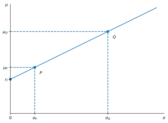
The CAL(Q) transforms risk into expected returns. It can be seen as a production function, just like the one we used in the Fisher model, where now the input is risk and the output is expected return. Thus, the Sharpe ratio of Q is the marginal rate of transformation (MRT) of risk into expected return. When Q is the market portfolio, this production function is exactly the CML.

Example 1 Suppose that r_{f} = 5\%, \mu_{Q} = 12\% and \sigma_{Q} = 20\%. The Sharpe ratio of Q is \mathit{SR} = \frac{0.12 - 0.05}{0.20} = 0.35.

Suppose that you want a portfolio P on the CAL(Q) but with 5% volatility. If w denotes the weight in Q, this means that 0.05 = w \times 0.20, or w = 25\%. Thus, a portfolio that invests 25% in Q and 75% in the risk-free asset has 5% volatility. The expected return of this portfolio is: \mu_{P} = 0.75 \times 0.05 + 0.25 \times 0.12 = 6.75\%. The position of P in the CAL(Q) is illustrated in Figure 1.

Example 2 Highland Capital Advisors (HCA) uses the capital market line to make asset allocation recommendations. HCA derives the following forecasts: an expected return on the market portfolio of \mu_{M} = 12\%, a standard deviation on the market portfolio of \sigma_{M} = 20\%, and a risk-free rate of r_{f} = 5\%.

Elena Cross seeks HCA’s advice for a portfolio asset allocation. Cross informs HCA that she wants the standard deviation of the portfolio to equal half of the standard deviation of the market portfolio. Using the capital market line, what expected return can HCA provide subject to Cross’s risk constraint?

Since the risky asset here is the market portfolio, the relevant investment opportunity set is the CML, whose slope is the Sharpe ratio already computed in Example 1, \mathit{SR} = 0.35. Cross’s risk constraint requires \sigma_{P} = 0.5 \times \sigma_{M} = 10.0\%. Plugging into the CML equation gives the expected return HCA can offer: \mu_{P} = r_{f} + \mathit{SR} \times \sigma_{P} = 0.05 + 0.35 \times 0.1 = 8.5\%. This portfolio invests w = \sigma_{P}/\sigma_{M} = 50.0\% in the market portfolio and the remaining 50.0\% in the risk-free asset.

Investor’s Utility

Investors seek to get the maximum return for the minimum risk. A standard way in economics to capture this trade-off is by using a utility function. The idea of introducing a utility function is to be able to rank different combinations of risk vs. return.

Recall from Utility Theory Under Uncertainty that a portfolio’s return is a proportional gamble on wealth, not a dollar gamble, and that for a small proportional gamble with mean \mu and variance \sigma^{2}, the certainty-equivalent return of a risk-averse investor is approximately \mu - \frac{1}{2}\mathit{RRA}\cdot \sigma^{2}, where \mathit{RRA} is the local coefficient of relative risk-aversion evaluated at the investor’s wealth. A simple and convenient way to model an investor’s preferences over portfolios is to promote this local approximation to a utility function defined over any (\mu, \sigma) pair, i.e., U(\mu, \sigma) = \mu - \frac{1}{2} A \sigma^{2}. \tag{3} Here A plays the same role as \mathit{RRA} did before: it denotes how sensitive is a particular investor to risk measured here by \sigma^{2}. A higher value for A reduces the utility for the same level of risk. We call A the coefficient of risk-aversion. It is common in applications to use values for A between 1 and 4.¹

¹ Unlike the local approximation above, which holds only approximately and only for small gambles, (3) can be obtained exactly from expected utility under exponential (CARA) utility, u(W) = -e^{-aW} as in Utility Theory Under Uncertainty, together with normally distributed portfolio returns. Let W_{0} be initial wealth and \tilde{r} \sim N(\mu, \sigma^{2}) the portfolio’s return, so that terminal wealth is \tilde{W} = W_{0}(1 + \tilde{r}). By the moment-generating function of the normal distribution, \operatorname{E}\left(e^{-aW_{0}\tilde{r}}\right) = e^{-aW_{0}\mu + \frac{1}{2}(aW_{0})^{2}\sigma^{2}}, so that \begin{aligned} \operatorname{E}(u(\tilde{W})) & = -e^{-aW_{0}} \operatorname{E}\left(e^{-aW_{0}\tilde{r}}\right) \\ & = -e^{-aW_{0}} \cdot e^{-aW_{0}\mu + \frac{1}{2}(aW_{0})^{2}\sigma^{2}} \\ & = -\exp\left[-aW_{0}\left((1 + \mu) - \frac{1}{2}(aW_{0})\sigma^{2}\right)\right]. \end{aligned} Since -e^{-x} is strictly increasing in x, ranking portfolios by expected utility is the same as ranking them by \mu - \frac{1}{2}(aW_{0})\sigma^{2}, which is exactly (3) with A = aW_{0}, the coefficient of relative risk-aversion \mathit{RRA} evaluated at W_{0}, consistent with the local argument above.

This means that there are several pairs (\mu, \sigma) that provide the same utility, i.e. for a given U and \sigma, we can always find a \mu such that: \mu = U + \frac{1}{2} A \sigma^{2}. These functions are called indifference curves since an investor with risk-aversion coefficient A is indifferent among any of these combinations of \mu and \sigma.

Let’s fix A = 3 and U to be either 2%, 6% or 10%. We can now plot the corresponding indifference curves.

Figure 2: The figure shows indifference curves for different levels of utility.

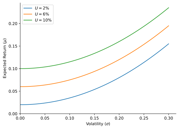
The curves in the graph represent all combinations of (\mu, \sigma) that provide the same utility, i.e. the investor is indifferent among these choices of risk and return. Indifference curves that provide higher utility are always above indifference curves that provide lower utility.

Each indifference curve can be characterized by its certainty equivalent, which represents the expected return that would provide the same level of utility with no risk, that is when \sigma = 0. The utility level can therefore be interpreted as the certainty equivalent of a particular portfolio.

Maximizing Utility

Optimal portfolio choice is about maximizing utility given the constraints imposed by the investment opportunity set. For a given w that determines the weight in the risk asset Q, the investment opportunity set is characterized by: \begin{aligned} \mu & = (1 - w) r_{f} + w \mu_{Q}, \\ \sigma^{2} & = w^{2} \sigma_{Q}^{2}. \end{aligned} \tag{4}

The utility of investing w in Q and the rest in the risk-free asset : \begin{aligned} U & = \mu - \frac{1}{2} A \sigma^{2} \\ & = (1 - w) r_{f} + w \mu_{Q} - \frac{1}{2} A w^{2} \sigma_{Q}^{2}. \end{aligned} The first-order condition (FOC) is: \frac{dU}{dw} = (\mu_{Q} - r_{f}) - A w \sigma_{Q}^{2} = 0. implying that the optimal w^{*} is given by: w^{*} = \frac{\mu_{Q} - r_{f}}{A \sigma_{Q}^{2}}.

The previous expression shows that the amount allocated to the risky asset is smaller if the risk aversion or if its variance are larger. We can see that in terms of allocation to the risky asset, the investor’s risk aversion and the variance of the asset play the same role and are indistinguishable. Certainly, we can also see that the amount allocated to the risky asset increases with its expected return, but decreases with the risk-free rate.²

² We will see later that if Q is the market portfolio, in equilibrium we must have that w^{*} = 1. Therefore, an increase in \sigma_{M}^{2} or A will translate in an increase of \mu_{M}, i.e. a decrease in prices.

Knowing w^{*} tells us how much to invest in the risky asset and therefore how much to invest in the risk-free asset. The resulting expected return and standard deviation of the optimal portfolio are given by: \begin{aligned} \mu^{*} & = (1 - w^{*}) r_{f} + w^{*} \mu_{Q}, \\ \sigma^{*} & = w^{*} \sigma_{Q}. \end{aligned}

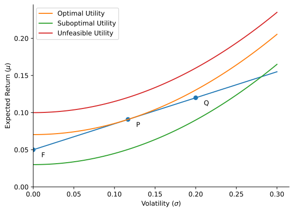
Example 3 Consider an agent with a risk-aversion coefficient equal to 3. If r_{f} = 5\%, \mu_{Q} = 12\% and \sigma_{Q} = 20\% as in Example 1, we have that w^{*} = \frac{0.12 - 0.05}{3 \times 0.20^{2}} = 58.33\%. Therefore, the portfolio that maximizes the utility for the investor consists of investing 41.67% in the risk-free asset and 58.33\% in the risky asset. The expected return and volatility of this portfolio are \begin{aligned} \mu^{*} & = (1 - w^{*}) \times 0.05 + w^{*} \times 0.12 = 9.08\%, \\ \sigma^{*} & = w^{*} \times 0.20 = 11.67\%. \end{aligned}

The optimal portfolio has the following interpretation. The investor wants to maximize utility, i.e., to achieve the highest level of utility possible. The point where the indifference curve is tangent to the CAL(Q) determines the optimal portfolio. At this point, the marginal rate of substitution between risk and return equals the marginal rate of transformation between risk and return — the same tangency condition that pinned down the optimal choice between consumption today and tomorrow in the Fisher model, only now applied to risk and return instead of C_{0} and C_{1}.

Figure 3: The figure shows that optimal portfolio choice occurs where the marginal rate of substituion equals the marginal rate of transformation between risk and return.

Practice Problems

These problems give you a chance to practice the concepts introduced in this chapter. Try to solve each one on your own before expanding the solution.

Problem 1 (Sharpe Ratio and Portfolio Weight) A brokerage forecasts a risk-free rate of r_{f} = 3\%, an expected return on the market portfolio of \mu_{M} = 11\%, and a market volatility of \sigma_{M} = 18\%. Compute the Sharpe ratio of the market portfolio. If a client wants a portfolio on the CML with 9\% volatility, what weight should she hold in the market portfolio, and what is the expected return of this portfolio?

Solution

The Sharpe ratio of the market portfolio is \mathit{SR} = \frac{\mu_{M} - r_{f}}{\sigma_{M}} = \frac{0.11 - 0.03}{0.18} = 0.4444. A portfolio with \sigma_{P} = 9\% requires a weight in the market portfolio of w = \frac{\sigma_{P}}{\sigma_{M}} = \frac{0.09}{0.18} = 50\%. Its expected return is \mu_{P} = r_{f} + \mathit{SR} \times \sigma_{P} = 0.03 + 0.4444 \times 0.09 = 7\%.

Problem 2 (Targeting an Expected Return on the CML) Using forecasts of r_{f} = 4\%, \mu_{M} = 10\%, and \sigma_{M} = 16\%, a client asks for a portfolio on the CML with an expected return of 8.5\%. What volatility does this portfolio have, and what weight does the client hold in the market portfolio?

Solution

The Sharpe ratio of the market portfolio is \mathit{SR} = \frac{0.10 - 0.04}{0.16} = 0.375. Setting \mu_{P} = r_{f} + \mathit{SR} \times \sigma_{P} equal to 8.5\% and solving for \sigma_{P} gives \sigma_{P} = \frac{0.085 - 0.04}{0.375} = 12\%. The corresponding weight in the market portfolio is w = \frac{\sigma_{P}}{\sigma_{M}} = \frac{0.12}{0.16} = 75\%.

Problem 3 (Computing Mean-Variance Utility) An investor with risk-aversion coefficient A = 4 is considering a portfolio with expected return \mu = 9\% and volatility \sigma = 15\%. Compute her utility level, and interpret it as a certainty equivalent.

Solution

Using (3), U = \mu - \frac{1}{2} A \sigma^{2} = 0.09 - \frac{1}{2} \times 4 \times 0.15^{2} = 4.5\%. The investor is indifferent between holding the risky portfolio and receiving a certain return of 4.5\%, which is her certainty equivalent for this portfolio.

Problem 4 (Certainty Equivalents and Points on an Indifference Curve) An investor with risk-aversion coefficient A = 2 has a certainty equivalent of CE = 5\% for her current portfolio, i.e., she is indifferent between holding it and receiving a sure return of 5\%. What expected return \mu must an alternative, riskier portfolio with \sigma = 10\% offer so that she is just as well off holding it instead?

Solution

Since the certainty equivalent is the expected return the investor would accept with no risk for the same utility, it equals her utility level, U = CE = 5\%. Any portfolio that delivers this same utility must lie on the corresponding indifference curve, \mu = U + \frac{1}{2} A \sigma^{2}, so at \sigma = 10\%, \mu = U + \frac{1}{2} A \sigma^{2} = 0.05 + \frac{1}{2} \times 2 \times 0.10^{2} = 6\%. The extra 1\% of expected return above the 5\% certainty equivalent is exactly the compensation this investor requires for bearing 10\% volatility.

Problem 5 (Optimal Capital Allocation) An investor with risk-aversion coefficient A = 4 faces r_{f} = 5\%, \mu_{Q} = 13\%, and \sigma_{Q} = 20\%. Find the optimal weight w^{*} in the risky asset, and the resulting expected return and volatility of the optimal portfolio.

Solution

Using the FOC, w^{*} = \frac{\mu_{Q} - r_{f}}{A \sigma_{Q}^{2}} = \frac{0.13 - 0.05}{4 \times 0.20^{2}} = 50\%. The expected return and volatility of the optimal portfolio are \begin{aligned} \mu^{*} & = (1 - w^{*}) \times 0.05 + w^{*} \times 0.13 = 9\%, \\ \sigma^{*} & = w^{*} \times 0.20 = 10\%. \end{aligned}

Problem 6 (Comparative Statics: Risk Aversion and Allocation) Two investors share the same forecasts, r_{f} = 5\%, \mu_{Q} = 13\%, and \sigma_{Q} = 20\%, but investor A has risk-aversion coefficient A = 2 while investor B has A = 8. Without recomputing everything from scratch, use the formula for w^{*} to predict how the two investors’ allocations to the risky asset should compare. Then verify your prediction by computing w^{*} for each investor.

Solution

Since w^{*} = \frac{\mu_{Q} - r_{f}}{A \sigma_{Q}^{2}} is inversely proportional to A for fixed forecasts, investor A (the less risk-averse of the two) should hold exactly 8/2 = 4 times the weight in the risky asset that investor B holds. Computing each, w^{*}_{A} = \frac{0.13 - 0.05}{2 \times 0.20^{2}} = 100\%, \qquad w^{*}_{B} = \frac{0.13 - 0.05}{8 \times 0.20^{2}} = 25\%, confirming that w^{*}_{A} / w^{*}_{B} = 4, as predicted.

Problem 7 (Optimal Allocation for a Client’s Portfolio) Assume that you manage a risky portfolio with an expected rate of return of 18\% and a standard deviation of 28\%. The T-bill rate is 8\%. Your client’s degree of risk aversion is A = 3.5, assuming a utility function U = \mu - 0.5 A \sigma^{2}.

1. What proportion of the total investment should be invested in your fund?
2. What is the expected return on your client’s optimized portfolio?
3. What is the standard deviation on your client’s optimized portfolio?

Solution

1. Using the FOC for optimal capital allocation, w^{*} = \frac{\mu_{Q} - r_{f}}{A \sigma_{Q}^{2}} = \frac{0.18 - 0.08}{3.5 \times 0.28^{2}} = \frac{0.10}{0.2744} \approx 36.44\%.

2. The expected return of the optimized portfolio is \mu^{*} = (1 - w^{*}) \times 0.08 + w^{*} \times 0.18 \approx 0.08 + 0.3644 \times 0.10 \approx 11.64\%.

3. The standard deviation of the optimized portfolio is \sigma^{*} = w^{*} \times 0.28 \approx 0.3644 \times 0.28 \approx 10.20\%.

Problem 8 (Indifference Curves and the Optimal Tangency Portfolio) Consider the following graph that plots four indifference curves of an investor with utility score given by U = \mu - 0.5 A \sigma^{2}. The indifference curves are labeled 1 through 4 in increasing order of utility, together with the capital allocation line (CAL) running from the risk-free asset F to the risky asset B. Curve 2 is tangent to the CAL at point P whereas curve 1 crosses the CAL at two points; curves 3 and 4 lie entirely above the CAL and never touch it.

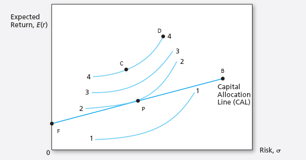
Currently, the investor can only invest in the risk-free asset denoted by F, and a risky asset denoted by B. You know that \mu_{B} = 11\%, \sigma_{B} = 15\%, and that the risk-free asset yields 5%.

1. Which indifference curve (1, 2, 3, or 4) represents the greatest level of utility that can be achieved by the investor? Why?
2. For which value of the risk-aversion coefficient would the optimal portfolio chosen by the investor be composed of 50% in the risky asset?

Solution

1. Curve 2 represents the highest utility the investor can actually attain. Curves 3 and 4 offer higher utility, but they lie entirely above the CAL and never touch it, so no combination of F and B can reach them — they describe levels of satisfaction that are unattainable given this investment opportunity set. Curve 1 is attainable, since it crosses the CAL twice, but it corresponds to lower utility than curve 2. Curve 2 is the highest indifference curve that is tangent to the CAL, at point P, so it is the best the investor can actually do.

2. The optimal weight in the risky asset is w^{*} = \dfrac{\mu_{B} - r_{f}}{A \sigma_{B}^{2}}. Setting w^{*} = 50\% and solving for A, A = \frac{\mu_{B} - r_{f}}{w^{*} \sigma_{B}^{2}} = \frac{0.11 - 0.05}{0.5 \times 0.15^{2}} = \frac{0.06}{0.01125} \approx 5.33.

Problem 9 (Client Portfolio Weights and the Sharpe Ratio) Assume that you manage a risky portfolio with an expected rate of return of 18\% and a standard deviation of 28\%. The T-bill rate is 8\%. Your client chooses to invest 70\% of a portfolio in your fund and 30\% in a T-bill money market fund.

1. What is the expected value and standard deviation of the rate of return on his portfolio?

2. Suppose that your risky portfolio includes the following investments in the given proportions:

   Asset	Proportions
   Stock A	25%
   Stock B	32%
   Stock C	43%

   What are the investment proportions of your client’s overall portfolio, including the position in T-bills?

3. What is the reward-to-volatility ratio, i.e. the Sharpe ratio, of your risky portfolio and your client’s portfolio?

Solution

1. Using (1) with w = 70\%, \mu_{P} = 0.7 \times 0.18 + 0.3 \times 0.08 = 15\%, \qquad \sigma_{P} = 0.7 \times 0.28 = 19.6\%.

2. Since the client holds 70\% of her wealth in the risky fund, her exposure to each of its underlying stocks is 70\% of that stock’s weight within the fund: 0.7 \times 25\% = 17.5\%, \qquad 0.7 \times 32\% = 22.4\%, \qquad 0.7 \times 43\% = 30.1\%. Her overall portfolio therefore consists of 17.5\% in Stock A, 22.4\% in Stock B, 30.1\% in Stock C, and the remaining 30\% in T-bills, which together sum to 100\%, as they must.

3. The Sharpe ratio of the risky portfolio is \mathit{SR}_{Q} = \frac{\mu_{Q} - r_{f}}{\sigma_{Q}} = \frac{0.18 - 0.08}{0.28} \approx 0.36, and the Sharpe ratio of the client’s overall portfolio is \mathit{SR}_{P} = \frac{\mu_{P} - r_{f}}{\sigma_{P}} = \frac{0.15 - 0.08}{0.196} \approx 0.36. Both are identical, since combining a risky portfolio with the risk-free asset moves you along the CAL(Q) without changing its slope: the Sharpe ratio only depends on the composition of the risky portfolio, not on how much of it you hold.