Perfect Correlation
Perfect correlation means one asset’s return is an exact linear function of the other’s, not approximately, but exactly. That exactness has a striking consequence: whether or not you can diversify away risk becomes a deliberate choice of weights rather than a byproduct of holding several assets. When two assets are perfectly negatively correlated, a long-only combination in the right proportions cancels their fluctuations completely. When they are perfectly positively correlated, no long-only combination helps at all, but going long one asset and short the other in the right proportion still drives risk exactly to zero.
This ability to build an exactly riskless portfolio out of risky assets is not just a mathematical curiosity. Because a riskless portfolio cannot earn anything other than the risk-free rate without creating an arbitrage opportunity, perfectly correlated assets pin down a synthetic risk-free rate implied by their prices. This same no-arbitrage logic, applied to an asset and an option written on it, is the foundation on which Black and Scholes (1973) and Merton (1973) built modern derivatives pricing.
The Zero Variance Portfolio
When the correlation between two risky assets A and B is either one or minus one, we say that the assets are perfectly correlated. In this case, it is possible to create a portfolio P between the two assets with zero variance.
We saw in the previous note that the variance of a portfolio in which we invest w_{A} in A and w_{B} in B is \sigma_{P}^{2} = w_{A}^{2} \sigma_{A}^{2} + w_{B}^{2} \sigma_{B}^{2} + 2 w_{A} w_{B} \sigma_{A, B}. \tag{1}
We start first considering the case where \rho_{A, B} = 1. In this case, we have that \sigma_{A, B} = \sigma_{A} \sigma_{B} and we can write equation (1) as \begin{aligned} \sigma_{P}^{2} & = w_{A}^{2} \sigma_{A}^{2} + w_{B}^{2} \sigma_{B}^{2} + 2 w_{A} w_{B} \sigma_{A} \sigma_{B} \\ & = (w_{A} \sigma_{A} + w_{B} \sigma_{B})^{2}. \end{aligned} \tag{2}
Since w_{A} = 1 - w_{B}, equation (2) can be made equal to zero by using w_{B} = \frac{\sigma_{A}}{\sigma_{A} - \sigma_{B}}.
Similarly, if \rho_{A, B} = -1, equation (1) implies that \sigma_{P}^{2} = (w_{A} \sigma_{A} - w_{B} \sigma_{B})^{2}. \tag{3} Substituting w_{A} = 1 - w_{B}, the previous expression can be made equal to zero if we pick w_{B} = \frac{\sigma_{A}}{\sigma_{A} + \sigma_{B}}. Therefore, we conclude that by picking w_{B} = \begin{cases} \dfrac{\sigma_{A}}{\sigma_{A} - \sigma_{B}} & \text{if $\rho_{A, B} = 1$}, \\ \dfrac{\sigma_{A}}{\sigma_{A} + \sigma_{B}} & \text{if $\rho_{A, B} = -1$}, \end{cases} \tag{4} and w_{A} = 1 - w_{B} we can make the variance of the portfolio equal to zero.
The portfolio characterized by w_{A} and w_{B} in (4) is the global minimum variance portfolio that achieves a variance equal to zero when the two assets are perfectly correlated. In probability, a random variable with zero variance must be constant. Thus, in the absence of arbitrage opportunities, the return of this portfolio must be equal to the risk-free rate. If not, you could borrow at a cheaper rate and invest at a higher rate without risk, generating arbitrarily large profits for free. Such a riskless profit would only last briefly in competitive financial markets.
Thus, we must have that r_{f} = \operatorname{E}(r_{P}) = w_{A} r_{A} + w_{B} r_{B}, \tag{5} where w_{B} is determined by equation (4) and w_{A} = 1 - w_{B}. The expression in (5) says that in the absence of arbitrage opportunities, it is possible to create your own risk-free asset if you can trade two perfectly correlated assets.
These assets typically do not exist as such in financial markets, but financial institutions can create them. For example, a call option is a contract that gives its purchaser the right but not the obligation to purchase an asset at a specific date in the future for a price agreed upon today. Call options exhibit positive perfect correlation with their underlying asset over short intervals. Thus, combining the underlying asset with a call option written on it can create an overnight risk-free asset. This remarkable insight allowed Black and Scholes (1973) and Merton (1973) to derive a formula for pricing derivatives!
A put option gives an example of an asset exhibiting a perfect negative correlation with an asset over short periods of time. A put gives its purchaser the right but not the obligation to sell an asset at a specific date in the future for a price agreed upon today. Again, combining the underlying asset with a put option written on it can create a risk-free asset. The idea of synthesizing a risk-free asset out of perfectly correlated risky assets has spawned a gigantic industry of derivatives products.
Example 1 (Perfect Positive Correlation) Suppose you have two risky assets A and B such that \mu_{A} = 14\%, \mu_{B} = 19\%, \sigma_{A} = 20\%, \sigma_{B} = 30\%, and \rho_{A, B} = 1.
We can use the expression for w_{B} defined in (4) to compute the implied risk-free rate. Thus, the portfolio defined by w_{B} = \frac{0.20}{0.20 - 0.30} = -2, and w_{A} = 1 - (-2) = 3 has zero variance. The implied risk-free rate is r_{f} = 3 \times 0.14 - 2 \times 0.19 = 4\%. We can verify that the variance of the portfolio is indeed zero, \sigma_{P} = 3 \times 0.2 -2 \times 0.3 = 0.
Example 2 (Perfect Negative Correlation) Suppose you have two risky assets A and B such that \mu_{A} = 13\%, \mu_{B} = -2\%, \sigma_{A} = 20\%, \sigma_{B} = 10\%, and \rho_{A, B} = -1.
We can use the expression for w_{B} defined in (4) to compute the implied risk-free rate. The portfolio characterized by w_{B} = \frac{0.20}{0.20 + 0.10} = 2/3, and w_{A} = 1/3, has zero variance. The implied risk-free rate is r_{f} = 1/3 \times 0.13 + 2/3 \times (-0.02) = 3\%. The variance of the portfolio is indeed zero since \sigma_{P} = 1/3 \times 0.2 - 2/3 \times 0.1 = 0.
Equation (5) can be written as w_{A} R_{A} + w_{B} R_{B} = 0, or R_{B} = \pm \frac{\sigma_{B}}{\sigma_{A}} R_{A}, \tag{6} where capital letters denote excess returns over the risk-free rate. The sign in equation (6) is the same as the correlation coefficient between the two assets. Thus, if two risky assets are perfectly correlated, their excess returns over the risk free rate must be proportional.
The Investment Opportunity Set
We just saw that we can make perfectly correlated assets out of a risky asset and the risk-free rate. Take a risky asset A with expected return equal to \mu_{A} and standard deviation equal to \sigma_{A}. \begin{aligned} \mu_{P} & = (1 - w) r_{f} + w \mu_{A}, \\ \sigma_{P} & = |w| \sigma_{A}. \end{aligned} Combining the previous two expressions, we find that the investment opportunity set of combining A and the risk-free asset is given by: \mu_{P} = \begin{cases} r_{f} + \left(\dfrac{\mu_{A} - r_{f}}{\sigma_{A}}\right) \sigma_{P} & \text{if $w > 0$}, \\ r_{f} - \left(\dfrac{\mu_{A} - r_{f}}{\sigma_{A}}\right) \sigma_{P} & \text{if $w < 0$}. \end{cases} \tag{8} The previous expression describes two lines that have the same intercept equal to the risk-free rate. The slope coefficient of the lines is equal to plus/minus the Sharpe ratio of asset A, depending on whether you invest or borrow asset A. This is the same capital allocation line from before, now recovered as a special case of combining two perfectly correlated assets. Figure 1 plots the investment opportunity set generated by asset A and the risk-free asset.
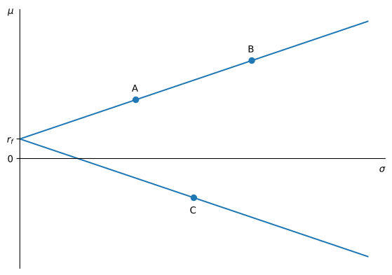
In the figure, the point B denotes a portfolio between A and the risk-free asset where R_{B} = w R_{A} and w > 1. Thus, assets A and B are perfectly positively correlated. If there was no risk-free asset, both risky assets could be combined together to create a risk-free asset.
Example 3 Suppose you have two risky assets A and B such that \mu_{A} = 15\%, \mu_{B} = 25\%, \sigma_{A} = 25\%, \sigma_{B} = 50\%, and \rho_{A, B} = 1.
This would be the situation described in Figure 1. The slope coefficient of the line created by A and B is \mathit{SR} = \frac{\mu_{B} - \mu_{A}}{\sigma_{B} - \sigma_{A}} = \frac{0.25 - 0.15}{0.50 - 0.25} = 0.40. The line between A and B is described by \mu = r_{f} + 0.40 \sigma, where r_{f} is the risk-free rate and represents the line intercept with the y-axis. The equation should be valid for both A and B, so we can pick either to compute the implied risk-free rate. If we use asset A we have that 0.15 = r_{f} + 0.40 \times 0.25, or r_{f} = 0.15 - 0.40 \times 0.25 = 5\%.
Practice Problems
These problems give you a chance to practice the concepts introduced in this chapter. Try to solve each one on your own before expanding the solution.
Problem 1 (A Zero-Variance Portfolio with Perfect Positive Correlation) Maya Lindqvist, compliance officer at the Ridgeway Teachers’ Pension Fund, is reviewing two structured notes written on the same equity index: the Index Growth Note (HGN) from Harbor Bank and the Index Plus Note (CSN) from Calder Securities. Because both notes pay off from the same index, their returns are perfectly positively correlated, \rho_{HGN, CSN} = 1. HGN offers expected return \mu_{HGN} = 16\% with volatility \sigma_{HGN} = 18\%, while CSN offers expected return \mu_{CSN} = 22\% with volatility \sigma_{CSN} = 27\%.
Before recommending either note to the fund’s board, Maya wants to check whether the two banks priced them consistently. A long position in one note and a short position in the other, in the right proportion, is riskless, so its return should equal the risk-free rate. Find the weights of this zero-variance portfolio and the risk-free rate it implies.
Solution
Using (4) with \rho_{HGN, CSN} = 1, w_{CSN} = \frac{\sigma_{HGN}}{\sigma_{HGN} - \sigma_{CSN}} = \frac{0.18}{0.18 - 0.27} = -2, so w_{HGN} = 1 - (-2) = 3. The fund would buy three dollars of HGN for every two dollars of CSN it sells short. By (5), the implied risk-free rate is r_{f} = 3 \times 0.16 - 2 \times 0.22 = 4\%. As a check, 3 \times 0.18 - 2 \times 0.27 = 0, confirming the portfolio has zero variance. If T-bills yield more or less than 4\%, the two notes are inconsistently priced.Problem 2 (A Zero-Variance Portfolio with an Inverse ETF) Individual stocks are almost never negatively correlated with one another, but an inverse ETF delivers negative correlation by construction. Owen Castillo, an analyst at Pemberton Capital, follows Corvane Robotics (CRV), which has expected return \mu_{CRV} = 11\% and volatility \sigma_{CRV} = 24\%. A sponsor has just listed the CRV -2\times ETF (CRVS), which delivers minus twice the return of CRV each period. Its volatility is therefore \sigma_{CRVS} = 48\%, its correlation with CRV is \rho_{CRV, CRVS} = -1, and Owen estimates its expected return at \mu_{CRVS} = -7\%.
Owen wants to combine CRV and CRVS into a portfolio with zero variance, a synthetic risk-free asset. Find the weights of this portfolio and the risk-free rate it implies.
Solution
Using (4) with \rho_{CRV, CRVS} = -1, w_{CRVS} = \frac{\sigma_{CRV}}{\sigma_{CRV} + \sigma_{CRVS}} = \frac{0.24}{0.24 + 0.48} = 1/3, so w_{CRV} = 2/3. Both weights are positive: with perfect negative correlation, a long-only portfolio is enough to eliminate risk. By (5), the implied risk-free rate is r_{f} = 2/3 \times 0.11 + 1/3 \times (-0.07) = 5\%. As a check, 2/3 \times 0.24 - 1/3 \times 0.48 = 0, confirming the portfolio has zero variance.Problem 3 (Two Funds on the Same Index) Priya Natarajan holds two ETFs from the same sponsor that track the same stock index: the Orchard Index ETF (ORC), with expected return \mu_{ORC} = 10\% and volatility \sigma_{ORC} = 16\%, and the Orchard 3\times Index ETF (ORX), with \mu_{ORX} = 22\% and \sigma_{ORX} = 48\%. Both funds move with the same index, so \rho_{ORC, ORX} = 1.
- Priya currently holds 50% in each fund. Compute the expected return and volatility of her portfolio.
- Show that any long-only mix of ORC and ORX has a volatility equal to the weighted average of the two funds’ volatilities, so it can never be less risky than ORC alone.
- Find the weights that eliminate risk entirely, and the risk-free rate they imply.
Solution
The expected return is 0.5 \times 0.10 + 0.5 \times 0.22 = 16\%. Since \rho_{ORC, ORX} = 1, equation (2) gives \sigma_{P} = 0.5 \times 0.16 + 0.5 \times 0.48 = 32\%.
By (2), \sigma_{P} = |w_{ORC} \sigma_{ORC} + w_{ORX} \sigma_{ORX}|. When both weights are nonnegative and sum to one, this is the weighted average w_{ORC} \times 16\% + w_{ORX} \times 48\%, which is at least 16\%. The cross term only lowers risk here when one of the positions is short.
Using (4), w_{ORX} = \frac{\sigma_{ORC}}{\sigma_{ORC} - \sigma_{ORX}} = \frac{0.16}{0.16 - 0.48} = -0.5, so w_{ORC} = 1.5. Priya would buy $1.50 of ORC for every $0.50 of ORX she sells short. The implied risk-free rate is r_{f} = 1.5 \times 0.10 - 0.5 \times 0.22 = 4\%.
Problem 4 (Proportional Excess Returns) Fenwick Biotech (FNB) has volatility \sigma_{FNB} = 25\%, and the FNB -2\times ETF (FNBD) has volatility \sigma_{FNBD} = 50\%, with \rho_{FNB, FNBD} = -1. The risk-free rate is 4\%. Daniel Okafor, who trades both, assumes markets are free of arbitrage.
- In a period in which FNB earns an excess return of 3\%, what excess return must FNBD earn? What is FNBD’s total return that period?
- Daniel holds the zero-variance portfolio of FNB and FNBD. Find its weights and verify that its excess return in that period is zero.
Solution
By (6), with the negative sign because \rho_{FNB, FNBD} = -1, R_{FNBD} = -\frac{\sigma_{FNBD}}{\sigma_{FNB}} R_{FNB} = -\frac{0.50}{0.25} \times 0.03 = -6\%. FNBD’s total return is r_{FNBD} = 0.04 - 0.06 = -2\%.
Using (4), w_{FNBD} = \frac{\sigma_{FNB}}{\sigma_{FNB} + \sigma_{FNBD}} = \frac{0.25}{0.25 + 0.50} = 1/3, so w_{FNB} = 2/3. The portfolio’s excess return is 2/3 \times 0.03 + 1/3 \times (-0.06) = 0, so it earns exactly the risk-free rate, as a riskless portfolio must.
Problem 5 (Hedging a Call Option) Pinecrest Options, a market maker, has sold call options on Halvorsen Shipping (HSC) to its clients. Over the next instant, the call’s return is perfectly positively correlated with the stock’s. HSC has expected return \mu_{HSC} = 12\% and volatility \sigma_{HSC} = 30\%, while the call has expected return \mu_{C} = 30\% and volatility \sigma_{C} = 120\%.
- Pinecrest hedges by combining the stock and the call into a zero-variance portfolio. Find the weights and the risk-free rate the hedge implies.
- T-bills currently yield 4\%. Show that Pinecrest can earn a riskless profit, and explain whether the call is overpriced or underpriced relative to the stock.
Solution
Using (4) with \rho = 1, w_{C} = \frac{\sigma_{HSC}}{\sigma_{HSC} - \sigma_{C}} = \frac{0.30}{0.30 - 1.20} = -1/3, so w_{HSC} = 4/3. Per dollar of capital, Pinecrest holds $1.33 of stock and is short $0.33 of calls, which matches its position as a seller of calls. The hedge earns 4/3 \times 0.12 - 1/3 \times 0.30 = 6\%.
The hedge earns a riskless 6\% while T-bills pay 4\%, so Pinecrest can borrow at 4\%, invest in the hedge, and keep 2\% per dollar borrowed. By (6), absence of arbitrage at r_{f} = 4\% requires \mu_{C} - r_{f} = \frac{\sigma_{C}}{\sigma_{HSC}} (\mu_{HSC} - r_{f}) = 4 \times 0.08 = 32\%, or \mu_{C} = 36\%. The call’s expected return of 30\% is too low, which means its price is too high: the call is overpriced, and the hedge profits by selling it. This is the no-arbitrage argument behind option pricing described at the start of this note.
Problem 6 (Insuring a Stock Position with Puts) The Alder Valley Endowment holds a large position in Granite Rail (GRR), with expected return \mu_{GRR} = 10\% and volatility \sigma_{GRR} = 20\%. The endowment’s treasurer, Hannah Brooks, considers buying put options on GRR. Over the next instant, the put’s return is perfectly negatively correlated with the stock’s, and the put has volatility \sigma_{\mathit{Put}} = 80\%. The risk-free rate is 4\%.
- What expected return must the put offer for markets to be free of arbitrage? Explain why it is negative.
- Find the weights of the zero-variance portfolio of GRR and puts, and verify that it earns the risk-free rate.
Solution
By (6), with the negative sign, \mu_{\mathit{Put}} - r_{f} = -\frac{\sigma_{\mathit{Put}}}{\sigma_{GRR}} (\mu_{GRR} - r_{f}) = -4 \times 0.06 = -24\%, so \mu_{\mathit{Put}} = -20\%. The put pays off when GRR falls, so it works as insurance. Buyers accept a negative expected return on it in exchange for that protection, just as homeowners pay insurance premiums that exceed expected claims.
Using (4), w_{\mathit{Put}} = \frac{\sigma_{GRR}}{\sigma_{GRR} + \sigma_{\mathit{Put}}} = \frac{0.20}{0.20 + 0.80} = 20\%, so w_{GRR} = 80\%. The portfolio earns 0.8 \times 0.10 + 0.2 \times (-0.20) = 4\%, the risk-free rate.
Problem 7 (Detecting an Arbitrage Opportunity) Lucas Ferreira, a junior trader at Whitcombe Securities, follows Ashford Water (AWC), with expected return \mu_{AWC} = 10\% and volatility \sigma_{AWC} = 12\%, and the AWC -1.5\times ETF (AWCS), which delivers minus one and a half times the return of AWC each period. AWCS has volatility \sigma_{AWCS} = 18\%, correlation \rho_{AWC, AWCS} = -1, and an expected return that Lucas estimates at \mu_{AWCS} = 1\%. The desk can borrow or lend at the risk-free rate of 5\%.
Lucas suspects that the right combination of AWC and AWCS lets the desk lock in a riskless profit at no cost. Determine whether such an arbitrage opportunity exists. If it does, explain how the desk should trade to exploit it, and compute the riskless profit per dollar borrowed.
Solution
Using (4) with \rho_{AWC, AWCS} = -1, w_{AWCS} = \frac{\sigma_{AWC}}{\sigma_{AWC} + \sigma_{AWCS}} = \frac{0.12}{0.12 + 0.18} = 40\%, so w_{AWC} = 60\%. This zero-variance portfolio has a certain return of 0.6 \times 0.10 + 0.4 \times 0.01 = 6.4\%, which exceeds the risk-free rate of 5\%. This is an arbitrage opportunity: borrow at 5\% and invest the proceeds 60\% in AWC and 40\% in AWCS, which pays a riskless 6.4\%. The desk earns 1.4\% of the amount borrowed with no net investment.Problem 8 (Creating Perfectly Correlated Assets Through Leverage) Sofia Marchetti, a trader at a proprietary trading desk, covers Northgate Semiconductor (NGS), with expected return \mu_{NGS} = 18\% and volatility \sigma_{NGS} = 22\%. The desk can borrow or lend freely at the risk-free rate of 4\%.
Her manager asks her to stress-test two strategies built entirely out of NGS and the risk-free asset, each placing weight w in NGS and 1 - w in the risk-free asset. For each strategy, find its expected return, its volatility, and the correlation between its excess return and that of NGS.
- A levered strategy L that borrows at the risk-free rate to invest w = 1.5 in NGS.
- A short strategy S that sells NGS short with w = -0.8 and invests the proceeds in the risk-free asset.
Solution
Each strategy has expected return r_{f} + w (\mu_{NGS} - r_{f}) and volatility |w| \sigma_{NGS}, and by (7) its excess return is w times that of NGS.
With w = 1.5, \mu_{L} = 0.04 + 1.5 \times (0.18 - 0.04) = 25\%, \qquad \sigma_{L} = 1.5 \times 0.22 = 33\%. Since w > 0, the excess returns of NGS and L are perfectly positively correlated, \rho_{NGS, L} = 1.
With w = -0.8, \mu_{S} = 0.04 + (-0.8) \times (0.18 - 0.04) = -7.2\%, \qquad \sigma_{S} = 0.8 \times 0.22 = 17.6\%. Since w < 0, the excess returns of NGS and S are perfectly negatively correlated, \rho_{NGS, S} = -1.
Problem 9 (Recovering the Risk-Free Rate from Two Correlated Funds) Grace Whitfield, an analyst at a consulting firm, is studying two funds run by Summit Asset Management: the Summit Equity Fund (SEF) and the Summit Leveraged Equity Fund (SLE), which holds the same stocks as SEF financed partly with borrowed money. Their returns are therefore perfectly positively correlated, \rho_{SEF, SLE} = 1. SEF has delivered an expected return \mu_{SEF} = 12\% with volatility \sigma_{SEF} = 15\%, while SLE has delivered \mu_{SLE} = 21\% with volatility \sigma_{SLE} = 40\%. Grace does not know the risk-free rate that prevailed when these figures were estimated, but she knows that perfectly correlated assets lie on the same straight line through the risk-free rate in (\sigma, \mu)-space.
Using only the data on SEF and SLE, find the slope of this line and the implied risk-free rate.