The Capital Asset Pricing Model
From Beta Pricing to the CAPM
Beta Pricing shows that the expected return of any asset A satisfies \operatorname{E}(r_{A}) = (1 - \beta_{A}) r_{f} + \beta_{A} \operatorname{E}(r_{Q}) for any mean-variance efficient portfolio Q. This result does not identify which portfolio is efficient, however. The Capital Asset Pricing Model (CAPM) supplies that missing link: in equilibrium, the efficient tangency portfolio Q is the market portfolio M.
This identification matters because constructing Q directly requires \pmb{w}_{Q} \propto \pmb{\Sigma}^{-1}(\pmb{\mu} - r_{f}\mathbf{1}). In practice, both inputs are difficult to estimate. Historical average returns are noisy estimates of \pmb{\mu}, and estimating and inverting a large covariance matrix \pmb{\Sigma} magnifies sampling error. Small changes in either input can therefore produce large changes in the estimated tangency weights.
Market-value weights do not require estimates of expected returns or covariances. The theoretical market portfolio nevertheless contains every risky asset in the investable universe, not just publicly listed stocks, so it is not observed exactly. In applications, investors use broad value-weighted indexes as proxies for M. The CAPM explains why the market portfolio, rather than a statistically estimated tangency portfolio, should be mean-variance efficient.
From Individual Choice to the Market Portfolio
The equilibrium argument rests on a short set of assumptions. Investors evaluate portfolios by their means and variances and share the same expected returns and covariance matrix (homogeneous expectations). They can trade the same assets without frictions, borrow or lend at a common risk-free rate, and choose portfolios in markets that clear. These assumptions connect individual portfolio choice to aggregate asset holdings.
Two-Fund Separation
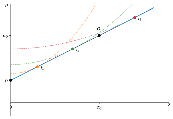
Recall from Optimal Capital Allocation that an investor with risk aversion A who combines the risk-free asset with a risky portfolio Q chooses weight w^{*} = \frac{\mu_{Q} - r_{f}}{A \sigma_{Q}^{2}} in Q. The weight w^{*} depends on risk aversion, but the composition of Q does not. Because investors have homogeneous expectations, they face the same efficient frontier and select the same risky portfolio with the highest Sharpe ratio. More risk-averse investors lend and hold less of Q; less risk-averse investors may borrow and hold more of it. In either case, they hold the risky assets in the same proportions. This result is the two-fund separation theorem.
Aggregation and Market Clearing
Let q_{j} be asset j’s weight in Q, and let W_{i} be investor i’s wealth. Investor i places w_{i}^{*} W_{i} q_{j} dollars in asset j. Summing across investors gives the aggregate demand for that asset: q_{j} \sum_{i} w_{i}^{*} W_{i}. The term multiplying q_j is the same for every risky asset. Consequently, the composition of aggregate risky-asset demand is exactly the composition of Q.
Market clearing requires investors collectively to hold the outstanding supply of every risky asset. If V_j denotes the total market value of asset j, its weight in aggregate risky wealth is \frac{V_j}{\sum_k V_k}. This is also asset j’s weight in the market portfolio M. Aggregate risky demand has Q’s composition and must equal aggregate risky supply, which has M’s composition. Therefore, Q = M.
This conclusion concerns the relative weights within the risky portfolio. It does not require the risk-free asset to be in zero net supply. A positive net supply of borrowing or lending instruments changes the fraction of aggregate wealth invested in risky assets, but not the relative weights of those risky assets.
The assumptions are restrictive. If investors disagree about expected returns or covariances, face different borrowing rates, or cannot trade the same assets, they need not choose the same tangency portfolio. Two-fund separation then fails at the aggregate level, and market clearing no longer implies that M is mean-variance efficient.
The CAPM Pricing Equation
Property 1 (The Capital Asset Pricing Model) If the assumptions of the CAPM hold, the market portfolio M is mean-variance efficient. The expected excess return of any asset A is therefore proportional to its market beta: \operatorname{E}(r_{A}) - r_f = \beta_A \bigl[\operatorname{E}(r_M) - r_f\bigr], \tag{1} where \beta_{A} = \frac{\operatorname{Cov}(r_{A}, r_{M})}{\operatorname{V}(r_{M})} measures the asset’s exposure to market risk.
Property 1 follows directly from the Beta Pricing proposition after equilibrium identifies Q with M. Equivalently, the CAPM expected-return equation can be written as \operatorname{E}(r_A) = r_f + \beta_A\bigl[\operatorname{E}(r_M)-r_f\bigr] = (1-\beta_A)r_f + \beta_A\operatorname{E}(r_M). The market risk premium \operatorname{E}(r_M)-r_f is the expected return investors require for bearing one unit of market risk. An asset with \beta_A=1 has the same expected excess return as the market, whereas an asset with \beta_A<1 has a smaller expected excess return. Idiosyncratic volatility does not enter the equation because it can be diversified away.
Example 1 (Computing a Stock Beta) Suppose the correlation between stock A and the market is 0.6. If the annual standard deviation of A’s return is 40% and the annual standard deviation of the market return is 20%, then \begin{aligned} \beta_{A} & = \frac{\operatorname{Cov}(r_{A}, r_{M})}{\operatorname{V}(r_{M})} = \frac{\sigma_{A} \sigma_{M} \rho_{A,M}}{\sigma_{M}^{2}} \\ & = \frac{\sigma_{A} \rho_{A,M}}{\sigma_{M}} = \frac{0.40 \times 0.60}{0.20} = 1.2. \end{aligned} A one-percentage-point change in the market return is associated with a 1.2-percentage-point change in A’s return through its systematic component.
Example 2 (Computing an Expected Return) If the risk-free rate is 5%, \beta_{DELL} = 1.3, and \operatorname{E}(r_M)=14\%, then the CAPM predicts \operatorname{E}(r_{DELL}) = 0.05 + 1.3(0.14-0.05) = 16.7\%. The 16.7% is Dell’s expected annual total return, including both price changes and distributions such as dividends. It is an average required return, not a guarantee of the return that will be realized next year.
Systematic and Firm-Specific Risk
Under the CAPM, an asset’s return can be decomposed into a systematic component linked to the market and a firm-specific, or idiosyncratic, component: r_A-r_f = \beta_A(r_M-r_f)+\varepsilon_A, \tag{2} where \operatorname{E}(\varepsilon_A)=0 and \operatorname{Cov}(\varepsilon_A,r_M)=0. The beta term captures systematic risk, which remains in a diversified portfolio. The residual \varepsilon_A captures firm-specific risk, which diversification can reduce.
This equation also explains how beta is estimated. A regression of an asset’s excess returns on the market’s excess returns has slope coefficient \beta_A = \frac{\operatorname{Cov}(r_A,r_M)}{\operatorname{V}(r_M)}. The regression residual estimates \varepsilon_A. In empirical work, the intercept is allowed to differ from zero so that researchers can test the CAPM rather than impose it.
Because the systematic and residual components are uncorrelated, the asset’s total variance is \sigma_{A}^{2} = \beta_{A}^{2} \sigma_{M}^{2} + \sigma^{2}(\varepsilon_{A}). \tag{3} The first term is systematic variance; the second is firm-specific variance. Only the exposure measured by \beta_A, not the amount of firm-specific variance, determines expected return under the CAPM.
Example 3 (Computing the Residual Risk) Suppose stock A has an annual return standard deviation of 40%, a market beta of 1.1, and the market has an annual return standard deviation of 20%. Its residual variance is \begin{aligned} \sigma^{2}(\varepsilon_A) &= \sigma_A^2-\beta_A^2\sigma_M^2 \\ &= 0.40^2-1.1^2(0.20^2) = 0.1116. \end{aligned} Therefore, the annual standard deviation of the firm-specific return is \sigma(\varepsilon_A)=\sqrt{0.1116}=33.41\%.
Interpreting Empirical Evidence
The CAPM is a statement about expected returns, which cannot be observed directly. Realized returns vary around their expectations, so a stock can earn more or less than the CAPM prediction over a particular month or year without violating the model. Empirical tests instead use many realized returns to estimate whether average returns are related to beta as the CAPM predicts.
A persistent deviation can have several interpretations. The asset may be mispriced, the market portfolio may not be mean-variance efficient because the CAPM’s assumptions fail, or the value-weighted index used by the researcher may be an imperfect proxy for the theoretical market portfolio. This market-proxy problem is central to Roll (1977): because the theoretical market portfolio cannot be observed, a test based on an index also tests whether that index is an adequate proxy for M.
This ambiguity is the joint-hypothesis problem: every empirical test of market efficiency is also a test of the asset-pricing model used to define the correct expected return. Rejecting the CAPM relation therefore rejects the combined hypothesis, not necessarily market efficiency alone.
Practice Problems
These problems give you a chance to practice the concepts introduced in this chapter. Try to solve each one on your own before expanding the solution.
Problem 1 (Two Investors, One Risky Portfolio) Nora Sato and Theo Lindgren are clients of the same advisor and share her forecasts. The tangency portfolio Q holds 50\% in Alder Technologies (ALD), 30\% in Birch Energy (BRE), and 20\% in Cobalt Health (CBH). It has expected return \mu_{Q} = 11\% and volatility \sigma_{Q} = 20\%, and T-bills yield 3\%. Nora has $200,000 and risk aversion A = 2; Theo has $500,000 and risk aversion A = 4.
- Compute each client’s optimal weight w^{*} in Q.
- How many dollars does each client invest in ALD, BRE, CBH, and T-bills?
- Compare the two clients’ holdings of the three stocks. What does the comparison illustrate?
- Suppose Nora and Theo were the only investors, and ALD, BRE, and CBH the only risky assets. What would the weights of the market portfolio be?
Solution
Using w^{*} = (\mu_{Q} - r_{f})/(A \sigma_{Q}^{2}), Nora holds 0.08/(2 \times 0.04) = 100\% in Q and Theo holds 0.08/(4 \times 0.04) = 50\%.
Nora invests all $200,000 in Q: $100,000 in ALD, $60,000 in BRE, $40,000 in CBH, and nothing in T-bills. Theo invests $250,000 in Q, split as $125,000 in ALD, $75,000 in BRE, and $50,000 in CBH, and the other $250,000 in T-bills.
Both clients hold the three stocks in the same 50 : 30 : 20 proportions. Risk aversion only determines how much of their wealth goes into Q and how much into T-bills, not which risky portfolio they hold. This is two-fund separation.
Together, Nora and Theo hold $225,000 in ALD, $135,000 in BRE, and $90,000 in CBH, out of $450,000 in stocks. Market clearing makes these the market values of the three companies, so the market weights are 50\%, 30\%, and 20\%, exactly the weights of Q. Because every investor holds the same risky portfolio, aggregate holdings have its composition, and the market portfolio is the tangency portfolio.
Problem 2 (Market Weights and Market Clearing) A small stock market lists three companies: Harlow Bank (HRB), with a market capitalization of $60 billion; Ives Motors (IVM), worth $30 billion; and Juno Media (JNM), worth $10 billion. Investors satisfy the assumptions of the CAPM.
- What are the weights of the tangency portfolio?
- Rafael Mendes has $1,000,000 and invests 80\% of it in the tangency portfolio. How much does he hold in each stock?
- The next day, Ives Motors’ share price rises 20\% and the other prices do not change. Compute the new market weights. Does Rafael need to trade to keep holding the market portfolio?
Solution
Under the CAPM, Q = M, so the tangency weights are the market-value weights. Total market value is $100 billion, giving 60\% in HRB, 30\% in IVM, and 10\% in JNM.
Rafael invests $800,000 in the market portfolio: $480,000 in HRB, $240,000 in IVM, and $80,000 in JNM. The remaining $200,000 goes to T-bills.
IVM is now worth $36 billion and the market $106 billion, so the weights become 60/106 \approx 56.6\%, 36/106 \approx 34.0\%, and 10/106 \approx 9.4\%. Rafael’s IVM position has also risen 20\%, so his stock holdings are in exactly these new proportions without any trade. A value-weighted portfolio rebalances itself as prices change.
Problem 3 (Finding Mispriced Stocks on the Security Market Line) Isabel Moreau, an analyst at Corran Partners, uses a risk-free rate of 4\% and an expected market return of 10\%. Her forecasts for three stocks are:
| Stock | Beta | Forecast Expected Return |
|---|---|---|
| Kestrel Airlines (KSA) | 1.4 | 13% |
| Linden Foods (LDF) | 0.7 | 7% |
| Mercer Steel (MCS) | 1.0 | 10% |
- Compute the expected return the CAPM requires for each stock, and the difference between Isabel’s forecast and that requirement.
- Which stocks plot above the security market line and which below? Which would Isabel consider underpriced?
Solution
By (1), with a market risk premium of 6\%, the required returns are \operatorname{E}(r_{KSA}) = 0.04 + 1.4 \times 0.06 = 12.4\%, \quad \operatorname{E}(r_{LDF}) = 0.04 + 0.7 \times 0.06 = 8.2\%, \quad \operatorname{E}(r_{MCS}) = 0.04 + 1.0 \times 0.06 = 10\%. The forecasts exceed these by +0.6\% for KSA, -1.2\% for LDF, and 0 for MCS.
KSA plots above the SML, LDF below it, and MCS on it. If Isabel’s forecasts are right, KSA offers more expected return than its market risk warrants, so it is underpriced. LDF offers less, so it is overpriced, and MCS is fairly priced. Whether KSA’s 0.6\% alpha is worth pursuing depends on how much firm-specific risk Isabel has to bear to collect it, a question the index model takes up.
Problem 4 (Beta and Residual Risk from a Regression) A regression of Ostrander Media’s (OSM) monthly excess returns on the market’s excess returns gives an R^{2} of 0.36 and a positive slope. OSM’s annual volatility is 40\%, the market’s is 20\%, the risk-free rate is 4\%, and the market risk premium is 6\%.
- Using the fact that R^{2} is the fraction of OSM’s variance explained by the market, compute OSM’s beta.
- Compute OSM’s firm-specific volatility \sigma(\varepsilon_{OSM}).
- What expected return does the CAPM assign to OSM? Does its firm-specific risk affect the answer?
Solution
By (3), R^{2} = \beta_{OSM}^{2} \sigma_{M}^{2} / \sigma_{OSM}^{2}, so \beta_{OSM} = \sqrt{R^{2}} \, \frac{\sigma_{OSM}}{\sigma_{M}} = 0.6 \times \frac{0.40}{0.20} = 1.2.
The residual variance is the unexplained fraction of total variance, \sigma^{2}(\varepsilon_{OSM}) = (1 - R^{2}) \sigma_{OSM}^{2} = 0.64 \times 0.16 = 0.1024, so \sigma(\varepsilon_{OSM}) = 32\%.
By (1), \operatorname{E}(r_{OSM}) = 0.04 + 1.2 \times 0.06 = 11.2\%. Firm-specific risk does not enter: most of OSM’s variance is firm-specific, but investors can diversify it away, so it earns no premium.
Problem 5 (The Cost of Capital for a New Project) Thalassa Petroleum (THP) has a beta of 1.4. It is considering a wind farm that costs $10 million today and is expected to pay $11 million in one year. Wind farms with long-term power contracts have a beta of about 0.8. The risk-free rate is 4\% and the market risk premium is 6\%.
- Compute the project’s NPV using the CAPM discount rate that matches the project’s risk.
- A manager proposes discounting the project at THP’s own cost of equity instead. What NPV does that give, and which decision is right?
Solution
The project’s required return is 0.04 + 0.8 \times 0.06 = 8.8\%, so \mathit{NPV} = \frac{11}{1.088} - 10 \approx \$0.110 \text{ million}.
THP’s cost of equity is 0.04 + 1.4 \times 0.06 = 12.4\%, which gives 11/1.124 - 10 \approx -\$0.214 million. The right discount rate reflects the risk of the project’s cash flows, not the risk of the firm that undertakes it, so THP should accept the project. Using the company-wide rate would reject a project that creates value for shareholders.
Problem 6 (Pricing a Stock with the CAPM) Analysts expect Penrose Instruments (PNI) to pay a dividend of $2 next year and to trade at $60 right after paying it. PNI’s beta is 1.25, the risk-free rate is 3\%, and the market risk premium is 7\%.
- What price should PNI trade at today?
- A change in PNI’s customer base raises its beta to 1.5, with the same expected cash flows. What happens to the price?
Solution
The required return is 0.03 + 1.25 \times 0.07 = 11.75\%. Discounting the expected dividend and price, P_{0} = \frac{2 + 60}{1.1175} \approx \$55.48.
The required return rises to 0.03 + 1.5 \times 0.07 = 13.5\%, so P_{0} = 62/1.135 \approx \$54.63. With the same expected cash flows, more market risk means a lower price today, and the lower price is what delivers the higher expected return.
Problem 7 (Diversifying Away Firm-Specific Risk) Wren Ellison builds an equally weighted portfolio of 20 stocks. Each stock has a beta of 1 and a firm-specific volatility of 30\%, and the residuals are uncorrelated across stocks. The market’s volatility is 18\%, the risk-free rate is 4\%, and the market risk premium is 6\%.
- Compute the volatility of a single stock and of the portfolio.
- Compute the expected return of a single stock and of the portfolio. Why does diversification lower risk without lowering expected return?
Solution
By (3), a single stock has variance 0.18^{2} + 0.30^{2} = 0.1224, or a volatility of about 35.0\%. The portfolio has beta 1, and its residual is the average of 20 uncorrelated residuals, with variance 0.09/20 = 0.0045. Its variance is 0.0324 + 0.0045 = 0.0369, a volatility of about 19.2\%.
Both have expected return 0.04 + 1 \times 0.06 = 10\%. The CAPM prices only market risk. The firm-specific risk that diversification removes earned no premium to begin with, so removing it costs nothing.
Problem 8 (Evaluating a Fund Manager) Over the past ten years, the Pryor Capital Opportunity Fund earned an average annual return of 14\% with a beta of 1.3 against the S&P 500. Over the same period, T-bills averaged 3\% and the S&P 500 averaged 10\%.
- What average return does the CAPM predict for the fund? Compute the fund’s alpha.
- The fund’s marketing materials claim the alpha proves the manager is skilled. Give three reasons the evidence might not support that claim.
Solution
The CAPM predicts 0.03 + 1.3 \times (0.10 - 0.03) = 12.1\%, so the fund’s alpha is 14\% - 12.1\% = 1.9\% a year.
First, realized returns vary around expected returns, and ten years of returns from a volatile stock fund leave a large sampling error, so the alpha may be luck. Second, the S&P 500 is only a proxy for the market portfolio; if it is not mean-variance efficient, the CAPM benchmark is wrong. Third, this is the joint-hypothesis problem: a positive alpha rejects the combination of the CAPM and the claim that prices are efficient, without saying which one fails. The fund may simply be earning a premium for a risk that the CAPM leaves out.
Solution
Setting w^{*} = (\operatorname{E}(r_{M}) - r_{f})/(A \sigma_{M}^{2}) = 1 gives \operatorname{E}(r_{M}) - r_{f} = A \sigma_{M}^{2} = 3 \times 0.18^{2} \approx 9.7\%.
The premium rises to 3 \times 0.22^{2} \approx 14.5\%. Expected cash flows do not change, so a higher expected return requires a lower price today: stock prices must fall until investors are again willing to hold the whole market.