Portfolios of Risky Assets
This chapter examines how combining risky assets shapes a portfolio’s risk and return. The central insight is that portfolio risk is not simply the average of its components’ risks: because asset returns do not move in lockstep, combining them can push risk below what any single asset offers on its own. This effect, known as diversification, is one of the most fundamental ideas in modern finance.
We begin with two risky assets to build intuition, deriving the investment opportunity set they generate and identifying the portfolio within it that achieves the lowest possible risk, the minimum-variance portfolio. We then examine how diversification behaves as more assets are added to a portfolio, and generalize the two-asset formulas to any number of risky assets using matrix notation. This will allow us to characterize the investment opportunity set achievable with many risky assets.
A Portfolio of Two Risky Assets
Suppose we have two risky assets A and B. The return of a portfolio P in which we invest 1 - w in A and w in B is r_{P} = (1 - w) r_{A} + w r_{B}. \tag{1} The expected return of the portfolio is \mu_{P} = (1 - w) \mu_{A} + w \mu_{B}, \tag{2} whereas its variance can be computed as \begin{aligned} \sigma_{P}^{2} & = \operatorname{V}((1 - w) r_{A} + w r_{B}) \\ & = (1 - w)^{2} \sigma_{A}^{2} + w^{2} \sigma_{B}^{2} + 2 w (1 - w) \sigma_{A, B}. \end{aligned} \tag{3} Here \sigma_{A, B} denotes the covariance of returns between A and B.
Example 1 (A Portfolio with Two Risky Assets) Consider two risky assets A and B for which you have the following information.
| Asset | Expected Return | Standard Deviation |
|---|---|---|
| A | 10% | 20% |
| B | 15% | 35% |
The correlation between the assets returns is 0.4. If you invest 40% in A and 60% in B, your portfolio will have an expected return of \mu = 0.4 \times 0.10 + 0.6 \times 0.15 = 13\%. Since the covariance of returns is \sigma_{AB} = 0.20 \times 0.35 \times 0.4 = 0.028, the standard deviation of the portfolio returns is \sigma = \sqrt{0.4^{2} \times 0.20^{2} + 0.6^{2} \times 0.35^{2} + 2 \times 0.4 \times 0.6 \times 0.028} = 25.29\%.
Suppose that now we want to vary w and see all the possible combinations of expected return (\mu_{P}) and standard deviation (\sigma_{P}) that we can obtain. In the previous example, we split the wealth between the two assets, so that 0 \leq w \leq 1 and 0 \leq 1 - w \leq 1. What if we wanted to invest more than 100% in asset B?
In financial markets, it is possible to borrow an asset and sell it immediately, a transaction known as short-selling the asset. There is typically no fixed date by which the asset must be returned to the lender; rather, it must be returned whenever the lender demands it.1
1 In practice, the lender (typically a broker) can recall the borrowed shares at their discretion, forcing the short-seller to buy them back on short notice. The short-seller must also compensate the lender for any dividends paid on the asset while the short position is open.
We assume throughout this class that short-selling is allowed. This means the weight w can be greater than one, in which case we short A to overinvest in B, or less than zero, in which case we short B to overinvest in A.
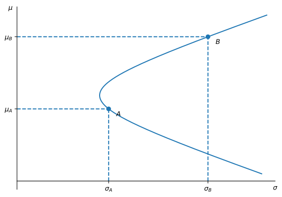
By varying w from -\infty to \infty, we obtain what is called the investment opportunity set generated by the two risky assets. If we plot \mu_{P} on the y-axis as a function of \sigma_{P} on the x-axis, the resulting figure is a hyperbola.
The Minimum Variance Portfolio (MVP)
As shown in the previous plot, there is a portfolio that has the minimum variance among all portfolios between A and B. To find its composition, we can use standard optimization techniques: \begin{aligned} \frac{d}{dw} \sigma_{P}^{2} & = \frac{d}{dw} (1 - w)^{2} \sigma_{A}^{2} + w^{2} \sigma_{B}^{2} + 2 w (1 - w) \sigma_{A, B} \\ & = - 2 (1 - w) \sigma_{A}^{2} + 2 w \sigma_{B}^{2} + 2 (1 - 2 w) \sigma_{A, B} = 0. \end{aligned} \tag{4} Thus, - (1 - w) \sigma_{A}^{2} + w \sigma_{B}^{2} + (1 - 2 w) \sigma_{A, B} = 0. or w_{MV} = \frac{\sigma_{A}^{2} - \sigma_{A, B}}{\sigma_{A}^{2} + \sigma_{B}^{2} - 2 \sigma_{A, B}}. \tag{5}
Property 1 (The Minimum Variance Portfolio) Given two risky assets A and B, there is a portfolio that has the minimum variance among all possible portfolios that can be built with A and B. The weights of the minimum variance portfolio are given by \begin{aligned} w_{A} & = \frac{\sigma_{B}^{2} - \sigma_{AB}}{\sigma_{A}^{2} + \sigma_{B}^{2} - 2 \sigma_{AB}}, \\ w_{B} & = \frac{\sigma_{A}^{2} - \sigma_{AB}}{\sigma_{A}^{2} + \sigma_{B}^{2} - 2 \sigma_{AB}}. \end{aligned} In the previous expression, \sigma_{A} and \sigma_{B} denote the standard deviation or volatility of returns. The term \sigma_{AB} denotes the covariance of A and B and is equal to \sigma_{AB} = \sigma_{A} \sigma_{B} \rho_{AB}, where \rho_{AB} is the correlation between the returns of A and B.
Example 2 (Minimum Variance Portfolio) Using the data of Example 1, we find that the weights of the minimum variance portfolio are given by \begin{aligned} w_{A} & = \frac{0.35^{2} - 0.028}{0.20^{2} + 0.35^{2} - 2 \times 0.028} = 88.73\% \\ w_{B} & = \frac{0.20^{2} - 0.028}{0.20^{2} + 0.35^{2} - 2 \times 0.028} = 11.27\% \end{aligned} Thus, the expected return and volatility of the minimum variance portfolio are \begin{aligned} \mu & = 0.8873 \times 0.10 + 0.1127 \times 0.15 = 10.56\%, \\ \sigma & = \sqrt{0.8873^{2} \times 0.20^{2} + 0.1127^{2} \times 0.35^{2} + 2 \times 0.8873 \times 0.1127 \times 0.028} \\ & = 19.66\%. \end{aligned}
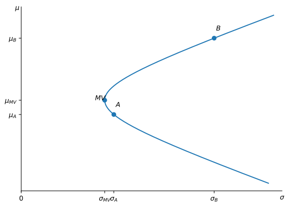
The MVP is the point farthest to the left of the investment opportunity set.
An Equally-Weighted Portfolio
The minimum-variance frontier demonstrates that combining two risky assets can alter the risk-return profile of the original assets. This concept is known as portfolio diversification.
To understand this phenomenon better, say that we have N securities and we invest the same amount in each, so the return of this portfolio (that we call P) is r_{P} = \frac{1}{N} \sum_{i = 1}^{N} r_{i}. The variance of P is given by \sigma_{P}^{2} = \frac{1}{N^{2}} \sum_{i = 1}^{N} \sum_{j = 1}^{N} \operatorname{Cov}(r_{i}, r_{j}). \tag{6}
The previous expression looks complex, but it is possible to decompose it into two intuitive parts. First, note that the average variance of the securities is given by \text{Avg. Variance} = \frac{1}{N} \sum_{i = 1}^{N} \operatorname{V}(r_{i}). Furthermore, the average covariance of the securities can be computed as \text{Avg. Covariance} = \frac{1}{N (N - 1)} \sum_{i = 1}^{N} \sum_{\substack{j = 1 \\ i \neq j}}^{N} \operatorname{Cov}(r_{i}, r_{j}) Using these two quantities, we can write (6) as \sigma_{P}^{2} = \frac{1}{N} (\text{Average Variance}) + \frac{N - 1}{N} (\text{Average Covariance}). \tag{7}
As N increases in (7), we have that \sigma_{P}^{2} \xrightarrow[N \rightarrow \infty]{} \text{Average Covariance}. The average variance disappears! This is the part of the risk that can be diversified away. What remains is the average covariance, which sets a floor on how much risk diversification can remove.
The 2008 financial crisis illustrated this limit. Correlations among mortgage-related assets that had appeared only loosely related rose sharply as the crisis unfolded, so portfolios that seemed well diversified suffered simultaneous losses.
A Portfolio of Many Risky Assets
The two-asset formulas above are a special case of a more general framework. Suppose there are N risky assets with returns r_{1}, r_{2}, \ldots, r_{N}. Collect the returns and the portfolio weights into vectors \mathbf{r} = \begin{pmatrix} r_{1} \\ r_{2} \\ \vdots \\ r_{N} \end{pmatrix}, \qquad \pmb{w} = \begin{pmatrix} w_{1} \\ w_{2} \\ \vdots \\ w_{N} \end{pmatrix}, where w_{i} is the fraction of wealth invested in asset i. Since short-selling is allowed, each w_{i} can be any real number, but the weights must still add up to the investor’s total wealth, \pmb{w}^{\top} \mathbf{1} = 1, \tag{8} where \mathbf{1} denotes the N-dimensional vector of ones. The portfolio return is the linear combination r_{P} = \pmb{w}^{\top} \mathbf{r} = \sum_{i = 1}^{N} w_{i} r_{i}. \tag{9}
By linearity of expectation, the expected return is \mu_{P} = \sum_{i=1}^{N} w_{i} \mu_{i} = \pmb{w}^{\top} \pmb{\mu}, where \pmb{\mu} = (\mu_{1}, \ldots, \mu_{N})^{\top} and \mu_{i} = \operatorname{E}(r_{i}). The variance, however, involves every pairwise covariance among the assets: writing r_{P} - \mu_{P} = \sum_{i} w_{i} (r_{i} - \mu_{i}) and squaring, \sigma_{P}^{2} = \operatorname{E}\left[ \left( \sum_{i = 1}^{N} w_{i} (r_{i} - \mu_{i}) \right)^{2} \right] = \sum_{i = 1}^{N} \sum_{j = 1}^{N} w_{i} w_{j} \operatorname{Cov}(r_{i}, r_{j}). This double sum is the N-asset generalization of (3); keeping track of its N variances and N(N - 1)/2 distinct covariances quickly becomes unwieldy as N grows.
Matrix notation packages this double sum compactly. Denote by \pmb{\Sigma} the covariance matrix of \mathbf{r}, the N \times N symmetric matrix whose (i,j) entry is \sigma_{ij} = \operatorname{Cov}(r_{i}, r_{j}), with \sigma_{ii} = \sigma_{i}^{2} on the diagonal. The double sum above is exactly the quadratic form \pmb{w}^{\top} \pmb{\Sigma} \pmb{w}, so \mu_{P} = \pmb{w}^{\top} \pmb{\mu}, \qquad \sigma_{P}^{2} = \pmb{w}^{\top} \pmb{\Sigma} \pmb{w}. \tag{10} The same expand-and-take-expectations argument, applied to the covariance of two different portfolios P and Q with weight vectors \pmb{w}_{P} and \pmb{w}_{Q}, gives2 \operatorname{Cov}(r_{P}, r_{Q}) = \pmb{w}_{P}^{\top} \pmb{\Sigma} \pmb{w}_{Q}, \tag{11} which reduces to (10) when Q = P.
2 For any weight vectors \pmb{a} and \pmb{b}, \operatorname{Cov}(\pmb{a}^{\top} \mathbf{r}, \pmb{b}^{\top} \mathbf{r}) = \sum_{i = 1}^{N} \sum_{j = 1}^{N} a_{i} b_{j} \operatorname{Cov}(r_{i}, r_{j}) = \pmb{a}^{\top} \pmb{\Sigma} \pmb{b}, by the same argument used above for \sigma_{P}^{2}.
3 With N = 2, set \pmb{w} = (1 - w, w)^{\top} and \pmb{\Sigma} = \begin{pmatrix} \sigma_{A}^{2} & \sigma_{A,B} \\ \sigma_{A,B} & \sigma_{B}^{2} \end{pmatrix}. Expanding the quadratic form gives \begin{aligned} \pmb{w}^{\top} \pmb{\Sigma} \pmb{w} & = \begin{pmatrix} 1 - w & w \end{pmatrix} \begin{pmatrix} \sigma_{A}^{2} & \sigma_{A,B} \\ \sigma_{A,B} & \sigma_{B}^{2} \end{pmatrix} \begin{pmatrix} 1 - w \\ w \end{pmatrix} \\ & = (1 - w)^{2} \sigma_{A}^{2} + w^{2} \sigma_{B}^{2} + 2 w (1 - w) \sigma_{A,B}, \end{aligned} which is exactly (3).
Equations (9) and (10) replace (2) and (3) for any number of assets, and collapse back to the two-asset formulas once N = 2.3
Example 3 (A Portfolio of Three Risky Assets) Consider three risky assets A, B, and C with the following expected returns and standard deviations.
| Asset | Expected Return | Standard Deviation |
|---|---|---|
| A | 8% | 15% |
| B | 12% | 20% |
| C | 15% | 25% |
The correlations between their returns are \rho_{AB} = 0.3, \rho_{AC} = 0.1, and \rho_{BC} = 0.4, so the covariance matrix is \pmb{\Sigma} = \begin{pmatrix} 0.0225 & 0.0090 & 0.00375 \\ 0.0090 & 0.0400 & 0.0200 \\ 0.00375 & 0.0200 & 0.0625 \end{pmatrix}.
If you invest \pmb{w} = (0.3, 0.3, 0.4)^{\top} in the three assets, (10) gives an expected return of \mu_{P} = \pmb{w}^{\top} \pmb{\mu} = 12.0\% and a variance of \sigma_{P}^{2} = \pmb{w}^{\top} \pmb{\Sigma} \pmb{w} = 0.0229, so that \sigma_{P} = 15.15\%. Computing \mu_{P} and \sigma_{P} only requires matrix multiplication, regardless of how many assets are in the portfolio.
The Investment Opportunity Set with Many Risky Assets
With two risky assets, tracing out (\sigma_{P}, \mu_{P}) as w ranges over all real numbers produces a single curve: each value of w pins down one portfolio, and there is exactly one free parameter to vary. With N risky assets, the weights \pmb{w} still have to satisfy the single budget constraint (8), which leaves N - 1 degrees of freedom. For N \geq 3, there are therefore many different portfolios that share the same expected return \mu_{P} but differ in variance \sigma_{P}^{2}. As a result, the set of achievable pairs (\sigma_{P}, \mu_{P}), the investment opportunity set, is no longer a curve but a filled two-dimensional region.
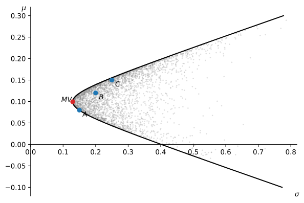
That region still has a well-defined left boundary, however. For each attainable level of expected return m, exactly one portfolio achieves it with the smallest possible variance; every other portfolio with that same expected return lies strictly to its right. Collecting these minimum-variance points as m varies traces out a curve called the minimum-variance frontier, and every portfolio in the investment opportunity set lies on or to the right of it.
We find the frontier by adding a target-return constraint to the variance minimization. For a target expected return m, we minimize \min_{\pmb{w}} \; \pmb{w}^{\top} \pmb{\Sigma} \pmb{w} \quad \text{subject to} \quad \pmb{w}^{\top} \mathbf{1} = 1 \quad \text{and} \quad \pmb{w}^{\top} \pmb{\mu} = m. Introducing a Lagrange multiplier for each constraint and following the same steps as for the minimum-variance portfolio4 gives a frontier variance of \sigma_{P}^{2}(m) = \frac{C m^{2} - 2 A m + B}{D}, \tag{12} where A = \pmb{\mu}^{\top} \pmb{\Sigma}^{-1} \mathbf{1}, \qquad B = \pmb{\mu}^{\top} \pmb{\Sigma}^{-1} \pmb{\mu}, \qquad C = \mathbf{1}^{\top} \pmb{\Sigma}^{-1} \mathbf{1}, \qquad D = BC - A^{2}. Equation (12) is a parabola in (\sigma_{P}^{2}, \mu_{P})-space, which is exactly why the frontier traces out a hyperbola in (\sigma_{P}, \mu_{P})-space, generalizing the hyperbola we found earlier with only two assets. Its minimum over m occurs at m = A / C, with \sigma_{P}^{2} = 1 / C = 1 / (\mathbf{1}^{\top} \pmb{\Sigma}^{-1} \mathbf{1}), which is the minimum-variance portfolio derived in the next section.
4 With two constraints, the Lagrangian is L(\pmb{w}, \lambda, \gamma) = \pmb{w}^{\top} \pmb{\Sigma} \pmb{w} - 2 \lambda (\pmb{w}^{\top} \pmb{\mu} - m) - 2 \gamma (\pmb{w}^{\top} \mathbf{1} - 1). The first-order condition gives \pmb{w} = \pmb{\Sigma}^{-1} (\lambda \pmb{\mu} + \gamma \mathbf{1}), and substituting into the two constraints yields the linear system \begin{pmatrix} B & A \\ A & C \end{pmatrix} \begin{pmatrix} \lambda \\ \gamma \end{pmatrix} = \begin{pmatrix} m \\ 1 \end{pmatrix}, so that \lambda = (Cm - A)/D and \gamma = (B - Am)/D. Plugging \pmb{w} back into \pmb{w}^{\top} \pmb{\Sigma} \pmb{w} = \lambda m + \gamma, using the two constraints, gives (12).
The figure below illustrates this for the three assets from Example 3. Each gray dot is a portfolio obtained by perturbing the equally-weighted portfolio with a random shock that is symmetric across the three assets and averages to zero, so the budget constraint continues to hold. Points near the frontier are denser than points far from it: moving away from the frontier at a fixed expected return raises the variance quadratically, so interior points require much larger short and levered positions.
The Minimum-Variance Portfolio with Many Risky Assets
With many risky assets, finding the minimum-variance portfolio means solving \min_{\pmb{w}} \; \pmb{w}^{\top} \pmb{\Sigma} \pmb{w} \quad \text{subject to} \quad \pmb{w}^{\top} \mathbf{1} = 1, i.e., minimizing (10) subject to the budget constraint (8). Introducing a Lagrange multiplier \lambda for the constraint, define the Lagrangian L(\pmb{w}, \lambda) = \pmb{w}^{\top} \pmb{\Sigma} \pmb{w} - 2 \lambda \left( \pmb{w}^{\top} \mathbf{1} - 1 \right), where the factor of 2 is just a convenient normalization for \lambda. The first-order condition with respect to \pmb{w} is5 2 \pmb{\Sigma} \pmb{w} - 2 \lambda \mathbf{1} = \mathbf{0} \quad \Longrightarrow \quad \pmb{w} = \lambda \pmb{\Sigma}^{-1} \mathbf{1}, where \pmb{\Sigma}^{-1} exists because \pmb{\Sigma} is positive definite: \pmb{w}^{\top} \pmb{\Sigma} \pmb{w} is the variance of the portfolio \pmb{w}, which is positive as long as no combination of the risky assets is riskless. Substituting into the budget constraint pins down the multiplier, \lambda \, \mathbf{1}^{\top} \pmb{\Sigma}^{-1} \mathbf{1} = 1 \quad \Longrightarrow \quad \lambda = \frac{1}{\mathbf{1}^{\top} \pmb{\Sigma}^{-1} \mathbf{1}}, which, substituted back, gives the following result.
5 Differentiating \pmb{w}^{\top} \pmb{\Sigma} \pmb{w} with respect to \pmb{w} gives 2 \pmb{\Sigma} \pmb{w} because \pmb{\Sigma} is symmetric, and differentiating \pmb{w}^{\top} \mathbf{1} gives \mathbf{1}.
Property 2 (The Minimum-Variance Portfolio with Many Assets) Given N risky assets with covariance matrix \pmb{\Sigma}, the minimum-variance portfolio has weights \pmb{w}_{MV} = \frac{\pmb{\Sigma}^{-1} \mathbf{1}}{\mathbf{1}^{\top} \pmb{\Sigma}^{-1} \mathbf{1}} \tag{13} and variance \sigma_{MV}^{2} = \frac{1}{\mathbf{1}^{\top} \pmb{\Sigma}^{-1} \mathbf{1}}. \tag{14}
To see why the variance takes this simple form, plug \pmb{w}_{MV} = \lambda \pmb{\Sigma}^{-1} \mathbf{1} into (10). Since \pmb{\Sigma} \pmb{w}_{MV} = \lambda \mathbf{1}, \sigma_{MV}^{2} = \pmb{w}_{MV}^{\top} \pmb{\Sigma} \pmb{w}_{MV} = \pmb{w}_{MV}^{\top} (\lambda \mathbf{1}) = \lambda \left( \pmb{w}_{MV}^{\top} \mathbf{1} \right) = \lambda, using the budget constraint \pmb{w}_{MV}^{\top} \mathbf{1} = 1 in the last step, which is exactly (14).
Equation (13) is the general version of (5): with N = 2 it reduces exactly to the weights w_{A} and w_{B} from Property 1.6
6 With N = 2 and \pmb{\Sigma} = \begin{pmatrix} \sigma_{A}^{2} & \sigma_{AB} \\ \sigma_{AB} & \sigma_{B}^{2} \end{pmatrix}, the formula for the inverse of a 2 \times 2 matrix gives \pmb{\Sigma}^{-1} \mathbf{1} = \frac{1}{\sigma_{A}^{2} \sigma_{B}^{2} - \sigma_{AB}^{2}} \begin{pmatrix} \sigma_{B}^{2} - \sigma_{AB} \\ \sigma_{A}^{2} - \sigma_{AB} \end{pmatrix}, so that \mathbf{1}^{\top} \pmb{\Sigma}^{-1} \mathbf{1} = \dfrac{\sigma_{A}^{2} + \sigma_{B}^{2} - 2 \sigma_{AB}}{\sigma_{A}^{2} \sigma_{B}^{2} - \sigma_{AB}^{2}}, and dividing each entry of \pmb{\Sigma}^{-1} \mathbf{1} by this quantity recovers exactly w_{A} and w_{B} from Property 1.
Example 4 (The Minimum-Variance Portfolio with Three Assets) Using the covariance matrix \pmb{\Sigma} from Example 3, (13) gives minimum-variance weights of 64.07\% in A, 19.05\% in B, and 16.88\% in C. This portfolio has an expected return of \mu_{MV} = 9.94\% and, by (14), a variance of \sigma_{MV}^{2} = 0.0168, i.e., a standard deviation of \sigma_{MV} = 12.95\%. Notice that \sigma_{MV} is lower than the volatility of any of the three individual assets, illustrating diversification with more than two risky assets.
The minimum-variance portfolio also satisfies a remarkable property, valid for any number of assets. Let \pmb{w}_{P} be the weights of an arbitrary portfolio P, so that \pmb{w}_{P}^{\top} \mathbf{1} = 1. By (11) and \pmb{w}_{MV} = \lambda \pmb{\Sigma}^{-1} \mathbf{1}, \operatorname{Cov}(r_{P}, r_{MV}) = \pmb{w}_{P}^{\top} \pmb{\Sigma} \pmb{w}_{MV} = \pmb{w}_{P}^{\top} \pmb{\Sigma} \left( \lambda \pmb{\Sigma}^{-1} \mathbf{1} \right) = \lambda \left( \pmb{w}_{P}^{\top} \mathbf{1} \right) = \lambda = \sigma_{MV}^{2}, using the budget constraint \pmb{w}_{P}^{\top} \mathbf{1} = 1 and (14) in the last two steps. The covariance of the MVP with any other portfolio is always the same and equal to its own variance! This also implies that the correlation of the MVP with any other portfolio is always positive, regardless of how many assets are in the investment universe.
Example 5 (Computing a Correlation with the MVP) Consider an investment opportunity set where the MVP has a standard deviation of returns of 20%. An asset A has a standard deviation of returns equal to 30%. Thus, \sigma_{A} \sigma_{MV} \rho_{A, MV} = \sigma_{A, MV} = \sigma_{MV}^{2}, or \rho_{A, MV} = \frac{\sigma_{MV}}{\sigma_{A}} = \frac{2}{3}.
Equations (5) and (13) demonstrate that the weights of the MVP depend solely on variances and covariances, which can typically be estimated with high precision from the data. In contrast, constructing any other portfolio within the investment opportunity set requires estimating expected returns, which are generally more challenging to estimate accurately. This is the reason why some practitioners like to use the MVP for their asset allocation. Moreover, forbidding short sales makes the estimated minimum-variance portfolio more robust. With fewer months of returns than stocks, the sample covariance matrix is singular and the textbook MVP does not exist; ruling out short sales removes the long-short positions that depend on the directions the data cannot pin down, so the problem has a solution. When the sample matrix is invertible, Jagannathan and Ma (2003) show that the constraint is equivalent to shrinking the largest covariance estimates, and that once short sales are ruled out, the sample covariance matrix performs as well as covariance matrix estimates based on factor models, shrinkage estimators, and daily data.
Practice Problems
These problems give you a chance to practice the concepts introduced in this chapter. Try to solve each one on your own before expanding the solution.
Problem 1 (Covariance and Correlation of Two Securities) Oliver Grant believes the economy has two equally likely states next month: boom (the good state) and recession (the bad state). At the beginning of the month, he can buy the following securities:
- Security 1 is a share of Sunvale Resorts (SVR), which trades at $4. Its price increases by $10 in the good state and remains unchanged in the bad state.
- Security 2 is a recession-protection contract sold by Bradwell Insurance, which trades at $5. It pays nothing extra in the good state and is worth $10 more in the bad state.
- Compute the expected returns of securities 1 and 2.
- Compute the standard deviations of returns for securities 1 and 2.
- Compute the covariance and the correlation between the returns of the two securities.
Solution
The HPRs in each state are r_{1}^{\text{good}} = \frac{10}{4} = 2.5, \quad r_{1}^{\text{bad}} = 0, \qquad r_{2}^{\text{good}} = 0, \quad r_{2}^{\text{bad}} = \frac{10}{5} = 2.
Since each state has probability 0.5, \mu_{1} = 0.5 \times 2.5 + 0.5 \times 0 = 1.25 = 125\%, \qquad \mu_{2} = 0.5 \times 0 + 0.5 \times 2 = 1 = 100\%.
The variances are \sigma_{1}^{2} = 0.5 (2.5 - 1.25)^{2} + 0.5 (0 - 1.25)^{2} = 1.5625, \qquad \sigma_{2}^{2} = 0.5 (0 - 1)^{2} + 0.5 (2 - 1)^{2} = 1, so \sigma_{1} = 1.25 = 125\% and \sigma_{2} = 1 = 100\%.
The covariance is \sigma_{12} = 0.5 (2.5 - 1.25)(0 - 1) + 0.5 (0 - 1.25)(2 - 1) = -1.25, so the correlation is \rho_{12} = \frac{\sigma_{12}}{\sigma_{1} \sigma_{2}} = \frac{-1.25}{1.25 \times 1} = -1. The securities move in opposite directions across states: when one gains, the other is flat. They are therefore perfectly negatively correlated. The negative correlation comes from the design of the insurance contract, which pays off exactly when the resort stock does badly; two ordinary stocks would rarely move against each other like this.
Problem 2 (Expected Return and Volatility of a Two-Asset Portfolio) Tomás Rivera is choosing between two mutual funds, the Dynamic Growth Fund (D) and the Emerging Opportunities Fund (E). Fund D is the steadier of the pair, with an expected return of \mu_{D} = 12\% and a volatility of \sigma_{D} = 18\%, while Fund E offers a higher expected return of \mu_{E} = 18\% but comes with substantially more risk, \sigma_{E} = 30\%. The two funds’ returns are only mildly related, with a correlation of \rho_{DE} = 0.25. He decides to build a portfolio that puts 60% of his wealth in D and the remaining 40% in E. What expected return and volatility should he expect from this portfolio?
Solution
Using (2), the expected return is \mu_{P} = 0.6 \times 0.12 + 0.4 \times 0.18 = 14.4\%. The covariance of returns is \sigma_{DE} = 0.18 \times 0.30 \times 0.25 = 0.0135, so using (3) the volatility is \sigma_{P} = \sqrt{0.6^{2} \times 0.18^{2} + 0.4^{2} \times 0.30^{2} + 2 \times 0.6 \times 0.4 \times 0.0135} = 18.04\%.Problem 3 (The Minimum-Variance Portfolio with Negatively Correlated Assets) Beatrice Hall holds shares of Anchor Steel Co. (STL), a stock with a volatility of \sigma_{STL} = 25\% whose returns have a correlation of 0.20 with the S&P 500. To offset some of that market exposure, she considers adding a leveraged inverse ETF (INV) designed to deliver twice the opposite of the index’s daily return. The ETF has a volatility of \sigma_{INV} = 40\%, and since it moves against the index, its correlation with STL is \rho_{STL, INV} = -0.20. Find the weights of the minimum-variance portfolio of STL and INV, and compute its volatility. Compare this volatility to \sigma_{STL} and \sigma_{INV}.
Solution
The covariance is \sigma_{STL, INV} = 0.25 \times 0.40 \times (-0.20) = -0.02. Using Property 1, w_{STL} = \frac{\sigma_{INV}^{2} - \sigma_{STL, INV}}{\sigma_{STL}^{2} + \sigma_{INV}^{2} - 2 \sigma_{STL, INV}} = \frac{0.16 - (-0.02)}{0.0625 + 0.16 - 2 \times (-0.02)} = 68.57\%, \qquad w_{INV} = 31.43\%. The variance of this portfolio is \sigma_{MV}^{2} = 0.6857^{2} \times 0.0625 + 0.3143^{2} \times 0.16 + 2 \times 0.6857 \times 0.3143 \times (-0.02) = 0.0366, so \sigma_{MV} = 19.12\%. This is lower than both \sigma_{STL} = 25\% and \sigma_{INV} = 40\%. Both weights are positive and the covariance is negative, so the cross term 2 w_{STL} w_{INV} \sigma_{STL, INV} subtracts from the variance. The negative correlation is built into the ETF, which delivers the opposite of the index’s return, rather than found between two stocks.Problem 4 (Diversification with Many Equally-Weighted Assets) Kenji Watanabe, a portfolio manager at Ravenhill Partners, follows a large universe of small biotechnology stocks, each with a variance of returns of 0.36 (i.e., a volatility of 60\%) and an average covariance between any two stocks of 0.09. If Kenji forms an equally-weighted portfolio of N = 25 of these stocks, what is the portfolio’s volatility? What volatility does the portfolio approach as N \to \infty, and what does this limit represent?
Solution
Using (7) with N = 25, \sigma_{P}^{2} = \frac{1}{25} \times 0.36 + \frac{24}{25} \times 0.09 = 0.1008, so \sigma_{P} = 31.75\%. As N \to \infty, the first term vanishes and \sigma_{P}^{2} \to 0.09, i.e., \sigma_{P} \to 30\%. This limit is the average covariance between the stocks: it represents the risk that cannot be diversified away, no matter how many stocks are added to the portfolio.Problem 5 (A Three-Asset Portfolio Using the Covariance Matrix) Priya Desai is building a portfolio out of three stocks that span a range of risk and return. Pembroke Utilities (PBU) is the most conservative of the three, with an expected return of \mu_{PBU} = 9\% and a volatility of \sigma_{PBU} = 12\%. Quarry Materials (QRM) sits in the middle, offering \mu_{QRM} = 14\% at a volatility of \sigma_{QRM} = 22\%. Zephyr Biotech (ZPB) is the most aggressive, with \mu_{ZPB} = 20\% and \sigma_{ZPB} = 30\%. The three stocks are not equally related to one another: PBU and QRM have a modest correlation of 0.2, PBU and ZPB are uncorrelated, and QRM and ZPB move together more closely, with a correlation of 0.5. Priya settles on the weights \pmb{w} = (0.5, 0.3, 0.2)^{\top} in PBU, QRM, and ZPB. Compute the expected return and volatility of the resulting portfolio.
Solution
The expected return is \mu_{P} = 0.5 \times 0.09 + 0.3 \times 0.14 + 0.2 \times 0.20 = 12.7\%. The covariance matrix is \pmb{\Sigma} = \begin{pmatrix} 0.0144 & 0.00528 & 0 \\ 0.00528 & 0.0484 & 0.033 \\ 0 & 0.033 & 0.09 \end{pmatrix}. Using (10), the variance is \sigma_{P}^{2} = \pmb{w}^{\top} \pmb{\Sigma} \pmb{w} = 0.0171, so \sigma_{P} = 13.08\%.Problem 6 (Correlation with the Minimum-Variance Portfolio) The Steadfast Minimum Volatility Fund holds the minimum-variance portfolio of a large stock universe, and its volatility is 15\%. Orrin Therapeutics (ORT), a biotech stock in that universe, is far more volatile, with a volatility of 45\%. What is the correlation between the returns of ORT and the returns of the fund?
Solution
Since \sigma_{ORT, MV} = \sigma_{MV}^{2} for every asset or portfolio in the universe, \rho_{ORT, MV} = \frac{\sigma_{ORT, MV}}{\sigma_{ORT} \sigma_{MV}} = \frac{\sigma_{MV}^{2}}{\sigma_{ORT} \sigma_{MV}} = \frac{\sigma_{MV}}{\sigma_{ORT}} = \frac{0.15}{0.45} = 33.33\%. Since every stock has the same covariance with the fund, the more volatile a stock is, the lower its correlation with the fund.Problem 7 (Comparative Statics: Correlation and Minimum-Variance Risk) Helena Brooks, the risk manager of the Marlow Foundation, wants to hold the minimum-variance mix of two funds, the Aldgate Fund (A) with a volatility of \sigma_{A} = 20\% and the Brookfield Fund (B) with \sigma_{B} = 30\%. Correlations between asset classes shift over time, and Helena’s estimate of the correlation between the two funds depends on the sample: data from one decade give \rho = -0.3, while data from another give \rho = 0.8.
- Compute the minimum-variance weights and volatility under each correlation estimate.
- Under which estimate is the minimum-variance portfolio less risky? Explain how each portfolio reduces risk, paying attention to the signs of the weights.
- Recompute the minimum-variance weights and volatility with \rho = 0.97. Does a lower correlation always lead to a less risky minimum-variance portfolio?
Solution
With \rho = -0.3, the covariance is \sigma_{AB} = 0.20 \times 0.30 \times (-0.3) = -0.018, so w_{A} = \frac{0.09 - (-0.018)}{0.04 + 0.09 - 2 \times (-0.018)} = 65.06\%, \qquad w_{B} = 34.94\%, and \sigma_{MV}^{2} = 0.6506^{2} \times 0.04 + 0.3494^{2} \times 0.09 + 2 \times 0.6506 \times 0.3494 \times (-0.018) = 0.0197, so \sigma_{MV} = 14.05\%. With \rho = 0.8, the covariance is \sigma_{AB} = 0.20 \times 0.30 \times 0.8 = 0.048, so w_{A} = \frac{0.09 - 0.048}{0.04 + 0.09 - 2 \times 0.048} = 123.53\%, \qquad w_{B} = -23.53\%, and \sigma_{MV}^{2} = 1.2353^{2} \times 0.04 + (-0.2353)^{2} \times 0.09 + 2 \times 1.2353 \times (-0.2353) \times 0.048 = 0.0381, so \sigma_{MV} = 19.52\%.
The minimum-variance portfolio is less risky under \rho = -0.3, with a volatility of 14.05\% against 19.52\%. With \rho = -0.3 it holds both funds long, and a negative covariance makes the cross term 2 w_{A} w_{B} \sigma_{AB} subtract from the variance. With \rho = 0.8 it shorts Fund B, so w_{A} w_{B} < 0, and a positive covariance also makes the cross term negative: the short position in B hedges part of the risk of A. At this correlation the hedge is not tight enough to beat the long-only mix.
With \rho = 0.97, the covariance is \sigma_{AB} = 0.20 \times 0.30 \times 0.97 = 0.0582, so w_{A} = \frac{0.09 - 0.0582}{0.04 + 0.09 - 2 \times 0.0582} = 233.82\%, \qquad w_{B} = -133.82\%, and \sigma_{MV}^{2} = 2.3382^{2} \times 0.04 + (-1.3382)^{2} \times 0.09 + 2 \times 2.3382 \times (-1.3382) \times 0.0582 = 0.0156, so \sigma_{MV} = 12.51\%. This is less risky than the long-only mix under \rho = -0.3, so the answer is no. As \rho approaches 1, the long-short hedge becomes nearly perfect, and at \rho = 1 the right weights make the portfolio riskless. How much risk the minimum-variance portfolio removes depends on the weights it can take given the correlation, not on the correlation alone.
Problem 8 (A Pension Fund’s Minimum-Variance Portfolio) Gloria Nash, who manages the Tri-County Firefighters’ Pension Fund, is considering two mutual funds from Crestline Investments: a stock fund and a long-term government and corporate bond fund. The probability distribution of the funds is as follows:
| Fund | Expected Return | Standard Deviation |
|---|---|---|
| Stock fund (S) | 20% | 30% |
| Bond fund (B) | 12% | 15% |
The correlation between the fund returns is 0.10.
What are the investment proportions in the minimum-variance portfolio of the two funds?
What is the expected value and standard deviation of the minimum-variance portfolio’s rate of return?
Compute the expected return and standard deviation of the following portfolios.
Proportion in S Proportion in B Expected Return Standard Deviation 25% 75% 50% 50% 75% 25%
Solution
The covariance between the funds is \sigma_{SB} = 0.30 \times 0.15 \times 0.10 = 0.0045. Using Property 1, w_{S} = \frac{\sigma_{B}^{2} - \sigma_{SB}}{\sigma_{S}^{2} + \sigma_{B}^{2} - 2 \sigma_{SB}} = \frac{0.0225 - 0.0045}{0.09 + 0.0225 - 2 \times 0.0045} = 17.39\%, \qquad w_{B} = 82.61\%.
Using (2) and (3) with these weights, \mu_{MV} = 0.1739 \times 0.20 + 0.8261 \times 0.12 = 13.39\%, \sigma_{MV} = \sqrt{0.1739^{2} \times 0.09 + 0.8261^{2} \times 0.0225 + 2 \times 0.1739 \times 0.8261 \times 0.0045} = 13.92\%. Note that \sigma_{MV} = 13.92\% is below the volatility of both the stock fund (30\%) and the bond fund (15\%). The correlation is positive, so with both funds held long the cross term adds a little variance, but each fund’s variance enters scaled by the square of its weight, and splitting the money between the two funds shrinks those terms by more.
Applying (2) and (3) to each pair of weights gives
Proportion in S Proportion in B Expected Return Standard Deviation 25% 75% 14% 14.13% 50% 50% 16% 17.43% 75% 25% 18% 23.18% For example, with 25\% in S and 75\% in B, \mu_{P} = 0.25 \times 0.20 + 0.75 \times 0.12 = 14\%, \sigma_{P} = \sqrt{0.25^{2} \times 0.09 + 0.75^{2} \times 0.0225 + 2 \times 0.25 \times 0.75 \times 0.0045} = 14.13\%, and analogously for the other two rows. As the weight shifts from B toward S, both the expected return and the volatility of the portfolio rise, since S has both a higher expected return and a higher standard deviation than B.
Problem 9 (Adding a Concentrated Stock Position) Daniel Reyes manages a $4,000,000 fully diversified portfolio for a client. The client unexpectedly receives a bonus of $1,000,000 in vested shares of her employer, Meridian Corp. Daniel has produced the following forecasts:
| Asset | Expected Return | Standard Deviation |
|---|---|---|
| Original Portfolio | 8.5% | 10% |
| Meridian Corp | 18% | 22% |
The correlation coefficient between Meridian Corp and the original portfolio is 0.30.
- The bonus changes the client’s overall portfolio, and she is deciding whether to keep the Meridian shares. Assuming she keeps them, calculate the expected return and standard deviation of her new $5,000,000 portfolio, which includes the Meridian shares.
- If she sells the Meridian shares, she will invest the proceeds in risk-free Treasury bills yielding 4.5%. Assuming she sells the shares and replaces them with the Treasury bills, calculate the expected return and standard deviation of her new portfolio.
- One of Daniel’s colleagues suggests that instead of buying Treasury bills, she sell the Meridian shares and use the $1,000,000 to buy shares of Atlas Corp, which has the same expected return and standard deviation as Meridian Corp. The colleague argues, “It doesn’t matter whether she keeps the Meridian shares or switches to Atlas instead.” State whether the colleague’s comment is correct or incorrect, and justify your answer briefly.
Solution
The client now holds 80\% of her wealth in the original portfolio and 20\% in Meridian Corp. The covariance between the two is \sigma_{OM} = 0.10 \times 0.22 \times 0.30 = 0.0066, so using (2) and (3), \mu_{P} = 0.8 \times 0.085 + 0.2 \times 0.18 = 10.4\%, \sigma_{P} = \sqrt{0.8^{2} \times 0.10^{2} + 0.2^{2} \times 0.22^{2} + 2 \times 0.8 \times 0.2 \times 0.0066} = 10.22\%.
Replacing Meridian Corp with a risk-free asset removes all covariance risk, so the portfolio is simply an 80/20 mix of the original portfolio and the risk-free rate, \mu_{P} = 0.8 \times 0.085 + 0.2 \times 0.045 = 7.7\%, \qquad \sigma_{P} = 0.8 \times 0.10 = 8\%.
The colleague’s comment is incorrect. Matching Meridian Corp’s expected return and standard deviation only pins down Atlas Corp’s own risk and return; it says nothing about how Atlas Corp moves together with the rest of the portfolio. The standard deviation of the combined position depends on the covariance, or equivalently the correlation, between the new stock and the original portfolio, not just on the new stock’s standalone volatility. Unless Atlas Corp also happens to share Meridian Corp’s 0.30 correlation with the original portfolio, switching into it will change \sigma_{P} even though \mu_{P} stays at 10.4\%.