Volatility Surface Modeling with Neural Networks

Introduction

In this notebook, I implement a neural network to model the implied volatility surface of SPX options. I load real-world options data, preprocess it, train a neural network to predict implied volatility based on key features, and evaluate its performance. Finally, I visualize the prediction errors with respect to moneyness and plot the volatility surface for a specific day.

The Black-Scholes model is one of the cornerstones of modern financial theory, providing a closed-form solution for pricing European-style options. However, in practice, market conditions can deviate from the assumptions of the Black-Scholes model, leading to discrepancies between theoretical and observed prices. Neural networks offer a flexible approach to model complex relationships in data, making them suitable for approximating option prices under various market conditions.

Data Loading and Preprocessing

I start by importing the core libraries used throughout the notebook. NumPy and pandas handle data transformations, matplotlib is used for plotting, PyTorch defines and trains the neural network, and scikit-learn provides preprocessing and evaluation tools. I also use yfinance to retrieve daily VIX levels, which act as a market-wide volatility feature.

import numpy as np
import matplotlib.pyplot as plt
import pandas as pd
import torch
import torch.nn as nn
from torch.utils.data import DataLoader, TensorDataset
from sklearn.model_selection import train_test_split
from sklearn.preprocessing import StandardScaler
from sklearn.metrics import mean_absolute_error, r2_score
import yfinance as yf

Before working with the data, I set seeds for reproducibility and select the compute device. This helps keep results stable across runs and automatically uses a GPU when available.

seed = 420
np.random.seed(seed)
torch.manual_seed(seed)
device = torch.device("cuda" if torch.cuda.is_available() else "cpu")

Next, I load the SPX option dataset and align it with VIX index values by date. The merge adds a market volatility state variable to each option observation. You can download the options file from here and place it in the same directory as this notebook.

df = pd.read_csv("./108105_2023_C_options_data.csv")
df["date"] = pd.to_datetime(df["date"])
vix = yf.download("^VIX", start="2023-01-01", progress=False, multi_level_index=False)[["Close"]]
vix.columns = ["^VIX"]
df = df.merge(vix, left_on="date", right_index=True, how="left")

This step applies data filters to remove extreme or noisy observations and then creates moneyness = K/S, which is one of the most informative features for IV surfaces. The filtering bounds focus the model on a realistic region of the surface used in class.

cleaned_df = df[["S", "K", "T", "Price", "^VIX", "Impl_Vol"]].copy()
cleaned_df = cleaned_df[(cleaned_df["Impl_Vol"] < 0.6) & 
                        (cleaned_df["T"] > 29) & 
                        (cleaned_df["T"] < 681)]
cleaned_df["moneyness"] = cleaned_df["K"] / cleaned_df["S"]
cleaned_df = cleaned_df[cleaned_df["moneyness"] > 0.1]

Model Training

Here I define the feature matrix X and target y, split into train/test sets, and standardize features using only the training sample. I convert arrays to PyTorch tensors and build a dataloader for mini-batch optimization. The train_size=0.01 choice is intentionally small for fast notebook execution; increasing it typically improves fit quality.

X = cleaned_df[["moneyness", "T", "S", "^VIX"]].values
y = cleaned_df["Impl_Vol"].values

X_train, X_test, y_train, y_test = train_test_split(X, y, train_size=0.01, random_state=seed)
scaler = StandardScaler()
X_train = torch.from_numpy(scaler.fit_transform(X_train)).float().to(device)
X_test = torch.from_numpy(scaler.transform(X_test)).float().to(device)
y_train = torch.from_numpy(y_train).float().to(device)
y_test = torch.from_numpy(y_test).float().to(device)

train_loader = DataLoader(TensorDataset(X_train, y_train), batch_size=64, shuffle=True)

I then define a feedforward network with two hidden ReLU layers. The model outputs one value per option: predicted implied volatility. I train it with Adam and use mean squared error as the objective.

model = nn.Sequential(
    nn.Linear(4, 256), nn.ReLU(),
    nn.Linear(256, 128), nn.ReLU(),
    nn.Linear(128, 1)
).to(device)

optimizer = torch.optim.Adam(model.parameters(), lr=1e-3, weight_decay=1e-4)
loss_fn = nn.MSELoss()

This loop performs gradient-based training for 40 epochs. At each batch, the code computes predictions, evaluates loss, backpropagates gradients, and updates weights. Printing every 5 epochs gives a quick diagnostic on whether optimization is progressing.

print("Training...")
for epoch in range(40):
    model.train()
    epoch_loss = 0.0
    for xb, yb in train_loader:
        optimizer.zero_grad()
        loss = loss_fn(model(xb).squeeze(), yb)
        loss.backward()
        optimizer.step()
        epoch_loss += loss.item()
    
    if epoch % 5 == 0:
        print(f"Epoch {epoch:02d} | Loss {epoch_loss / len(train_loader):.8f}")

Training...
Epoch 00 | Loss 0.00217907
Epoch 05 | Loss 0.00007633
Epoch 10 | Loss 0.00006824
Epoch 15 | Loss 0.00005860
Epoch 20 | Loss 0.00005644
Epoch 25 | Loss 0.00005957
Epoch 30 | Loss 0.00006065
Epoch 35 | Loss 0.00006338

Model Evaluation

After training, I evaluate out-of-sample accuracy on the test set. I report MAE, RMSE, and R-squared to summarize typical pricing error magnitude and overall explanatory power.

model.eval()
with torch.no_grad():
    y_pred = model(X_test).squeeze().cpu().numpy()
y_true = y_test.cpu().numpy()

mae = mean_absolute_error(y_true, y_pred)
rmse = np.sqrt(np.mean((y_pred - y_true)**2))
r2 = r2_score(y_true, y_pred)
print(f"\nTest - MAE: {mae:.6f} | RMSE: {rmse:.6f} | R²: {r2:.6f}")

Test - MAE: 0.004617 | RMSE: 0.006896 | R²: 0.969675

The next two figures give a visual diagnostic of model quality. The first plot shows how absolute prediction error varies with moneyness; the second compares predicted versus observed implied volatility and overlays a 45-degree reference line.

moneyness_test = scaler.inverse_transform(X_test.cpu().numpy())[:, 0]
abs_err = np.abs(y_pred - y_true)

fig, ax = plt.subplots(figsize=(8, 5))
ax.scatter(moneyness_test, abs_err, alpha=0.5, s=1, rasterized=True)
ax.set(
    xlabel="Moneyness (Strike / Spot)",
    ylabel="Absolute IV Error",
    title=f"Absolute Implied Volatility Error vs Moneyness (MAE={mae:.4f})",
)
ax.grid(True, alpha=0.3)
plt.tight_layout()
plt.show()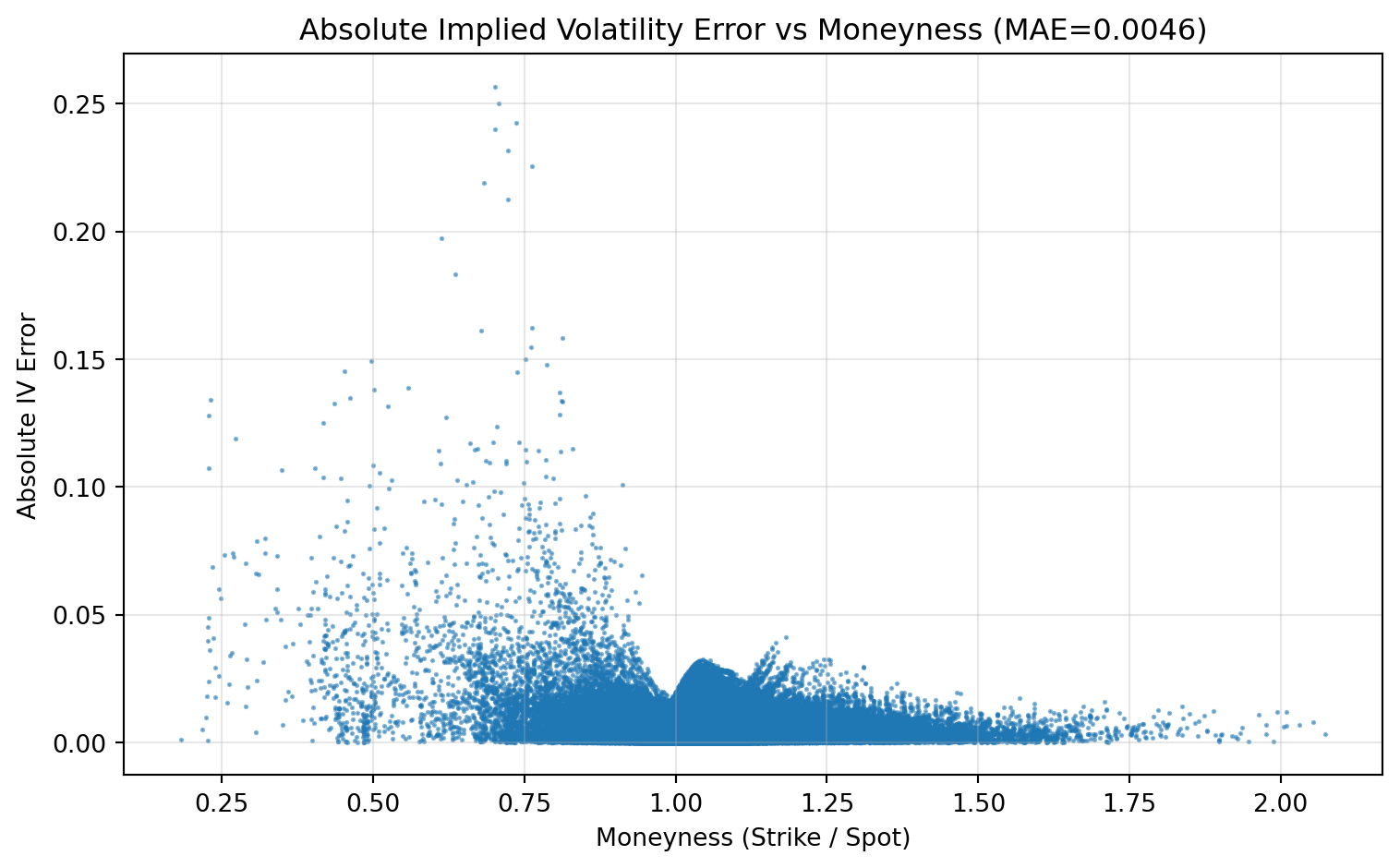

fig, ax = plt.subplots(figsize=(8, 5))
ax.scatter(y_true, y_pred, alpha=0.5, s=1, rasterized=True)
ax.plot([y_true.min(), y_true.max()], [y_true.min(), y_true.max()], "r--", lw=2)
ax.set(
    xlabel="Observed Implied Volatility",
    ylabel="Predicted Implied Volatility",
    title=f"Predicted vs Observed Implied Volatility (R²={r2:.4f})",
)
ax.grid(True, alpha=0.3)
plt.tight_layout()
plt.show()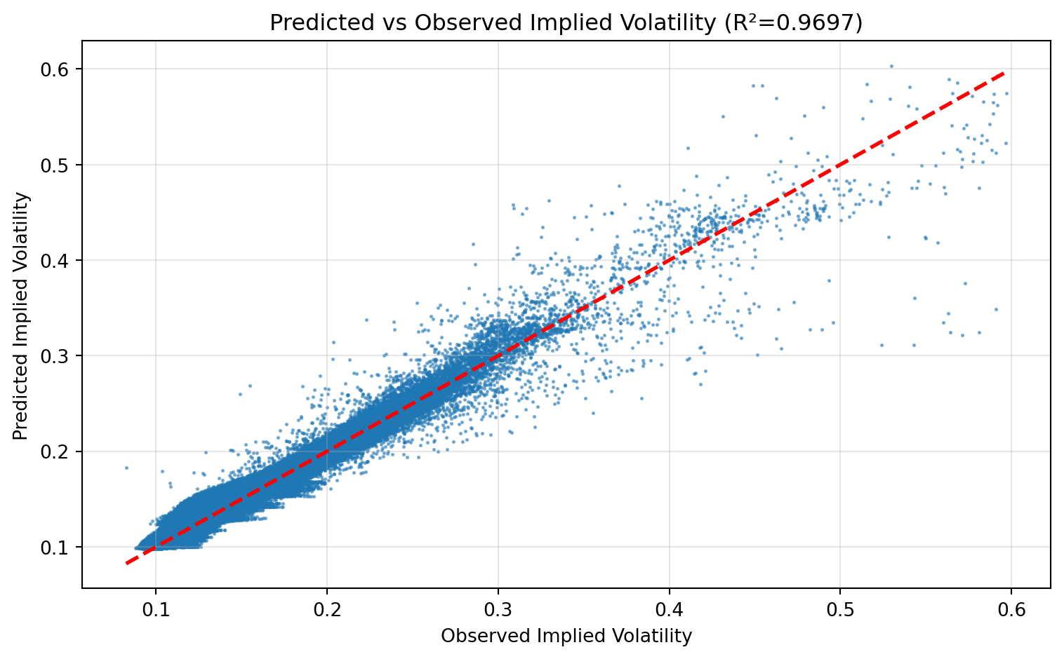

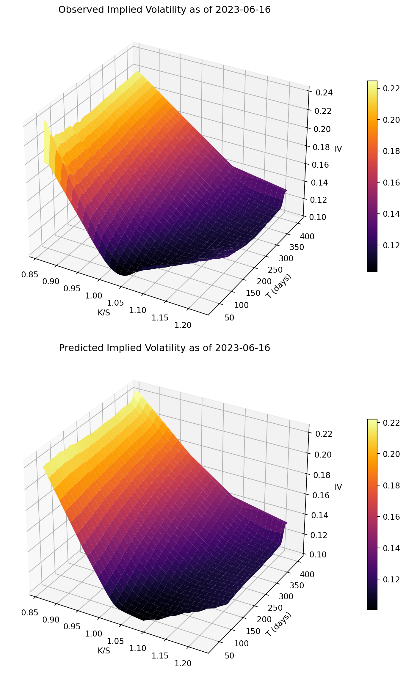
Visualizing the Volatility Surface

To inspect cross-sectional fit more directly, I compare observed and predicted IV surfaces for one day.

from scipy.interpolate import griddata

I first reconstruct a clean analysis dataset using the same filters as the model section and create moneyness.

tmp = (
    df[["date", "S", "K", "T", "^VIX", "Impl_Vol"]]
    .dropna()
    .assign(date=lambda x: pd.to_datetime(x["date"]), moneyness=lambda x: x["K"] / x["S"])
    .query("Impl_Vol < 0.6 and T > 29 and T < 681 and moneyness > 0.1")
)

I then select the trading date closest to June 16, 2023, which keeps the notebook robust when the exact timestamp is missing.

target = pd.Timestamp("2023-06-16")
dates = pd.to_datetime(tmp["date"].unique())
day = dates[np.argmin(np.abs((dates - target).to_numpy()))]
d = tmp[tmp["date"] == day].copy()
if d.empty:
    raise ValueError(f"No data available near {target.date()} after filters")

Next, I generate model predictions for that day’s option contracts. Inputs are scaled with the same scaler fitted on training data.

X_day = d[["moneyness", "T", "S", "^VIX"]].to_numpy(dtype=np.float32)
with torch.no_grad():
    iv_pred = model(torch.from_numpy(scaler.transform(X_day)).to(device)).squeeze(-1).cpu().numpy()

m = d["moneyness"].to_numpy()
T = d["T"].to_numpy()
iv_obs = d["Impl_Vol"].to_numpy()

I then interpolate scattered observations onto a regular (moneyness, maturity) grid to make side-by-side surface plots easier to compare.

mg = np.linspace(np.quantile(m, 0.02), np.quantile(m, 0.98), 60)
Tg = np.linspace(np.quantile(T, 0.02), np.quantile(T, 0.98), 60)
MM, TT = np.meshgrid(mg, Tg)

Zobs = griddata(np.c_[m, T], iv_obs, (MM, TT), method="linear")
Zpred = griddata(np.c_[m, T], iv_pred, (MM, TT), method="linear")

Finally, I render two 3D surfaces with a common colormap: observed IV and predicted IV for the same day. Visual agreement in level and shape indicates the network captures the main surface structure.

fig = plt.figure(figsize=(8, 12))
for i, (Z, title) in enumerate([(Zobs, "Observed Implied Volatility as of"), (Zpred, "Predicted Implied Volatility as of")], start=1):
    ax = fig.add_subplot(2, 1, i, projection="3d", rasterized=True)
    surf = ax.plot_surface(MM, TT, Z, cmap="inferno", linewidth=0, antialiased=True)
    ax.set(
        title=f"{title} {day.date()}",
        xlabel="K/S",
        ylabel="T (days)",
        zlabel="IV",
    )
    fig.colorbar(surf, ax=ax, shrink=0.6, pad=0.1)

plt.tight_layout()
plt.show()