b = "hello".encode("utf-8")

for byte in b:
    print(format(byte, '08b'))
01101000
01100101
01101100
01101100
01101111A computer represents characters as bytes (8 bits). For example, the string “hello” consists of 5 characters encoded as 5 bytes. Binary digits (bits) are an alternative to decimal for representing numbers. A byte is a group of 8 bits; for instance, the binary byte 10101100 (which in ASCII corresponds to the character ¬) equals
1 \cdot 2^7 + 0 \cdot 2^6 + 1 \cdot 2^5 + 0 \cdot 2^4 + 1 \cdot 2^3 + 1 \cdot 2^2 + 0 \cdot 2^1 + 0 \cdot 2^0 = 172
in decimal. In hexadecimal notation, this byte is AC because
10 \cdot 16^1 + 12 \cdot 16^0 = 160 + 12 = 172.
Thus,
10101100_2 =\text{AC}_{16} = 172_{10}.
Since each hex digit represents 4 bits, two hex digits correspond to one byte. A 256-bit hash thus becomes a 64-character hexadecimal string:
256 \text{ bits} = 32 \text{ bytes} = 64 \text{ hex characters}.
Hexadecimal is widely used in cryptography for its compact, human-readable representation of binary data.1 In the context of blockchain, hexadecimal is commonly used to represent hashes, addresses, and other binary data in a human-readable format. In UTF-8 encoding, the string “hello” is represented as the byte sequence 68 65 6C 6C 6F in hexadecimal, where each pair of hex characters corresponds to one character in the string.
1 In the beginning of the computer age, programmers worked directly with hexadecimal values using punch cards or hexadecimal input devices, making coding error-prone and requiring deep hardware knowledge. Modern encoding methods like UTF-8 have since abstracted away these low-level details. However, hexadecimal remains important for applications like cryptography, where compact and precise representation of binary data is crucial.
For example, the following code shows how the string “hello” is converted to bytes:
b = "hello".encode("utf-8")
for byte in b:
print(format(byte, '08b'))01101000
01100101
01101100
01101100
01101111The encode method converts the string into bytes, which can then be used for hashing or other binary operations. The format(byte, '08b') function formats each byte as an 8-bit binary string, padding with zeros if necessary. This illustrates how the string “hello” is represented in binary form before being processed by a hash function like SHA-256. To see the actual byte values in hexadecimal, you can use the hex method on the byte object:
"hello".encode("utf-8").hex()'68656c6c6f'A hash function is a mathematical algorithm that takes an input (or “message”) and produces a fixed-size string of bytes, typically a hexadecimal number. The output is called the hash or digest. Hash functions have several key properties:
Bitcoin and many other applications use the SHA-256 hash function which produces a 256-bit (32-byte) hash, typically represented as a 64-character hexadecimal string. Note that 256 bits can represent a decimal number with up to 78 digits, which is comparable to the number of atoms in the observable universe, making it effectively impossible to brute-force search for collisions or pre-images.
Hash functions are fundamental to Bitcoin’s security and structure, enabling the creation of a tamper-evident ledger and the proof-of-work (PoW) mechanism. But hash functions are also widely used in other contexts, such as software or file integrity checks. If you want to make sure an installation file hasn’t been altered by hackers, you can compute its hash and compare it to a known good value. If the hashes match, the file is likely unchanged; if they differ, the file may have been modified or corrupted.
If you download the current version of Python from the official website, you can find the SHA-256 hash of the installer file listed on the download page. After downloading, you can compute the hash of the file on your computer and compare it to the provided hash to ensure the file’s integrity.
In Python, you can compute a SHA-256 hash using the hashlib library. The function sha256_hex below takes a string input and returns its SHA-256 hash in hexadecimal format.
import hashlib

def sha256_hex(s):
    return hashlib.sha256(s.encode("utf-8")).hexdigest()
This function encodes the input string to bytes (using UTF-8 encoding) before hashing, which is necessary because the SHA-256 algorithm operates on byte data. The function hashlib.sha256() always outputs 256 bits, which is 32 bytes. The function hexdigest() converts those bytes into a hexadecimal string, which is why we get a 64-character string as the output (since each byte corresponds to two hex characters).
For example, sha256_hex("hello world") will return the hash of the string “hello world”:
print(sha256_hex("hello world"))b94d27b9934d3e08a52e52d7da7dabfac484efe37a5380ee9088f7ace2efcde9Note how different the hash is if we now use “Hello World” (capitalized):
print(sha256_hex("Hello World"))a591a6d40bf420404a011733cfb7b190d62c65bf0bcda32b57b277d9ad9f146eBitcoin is a distributed payment system with no central ledger manager, so the main problem is coordination: independent nodes must agree on one transaction history even when messages are delayed and some participants are malicious.
The process starts with transactions. A Bitcoin transaction is a signed message that spends previously received coins and assigns them to new owners. Users broadcast transactions to the peer-to-peer network, and nodes validate them against protocol rules before relaying them.
Miners gather valid transactions into candidate blocks. Each block has a body (the transactions) and a header (metadata used for identification and PoW). In this simplified view, the header contains the previous block hash, a transaction summary (typically a Merkle root), a timestamp, and a nonce.
The Merkle root is a single hash that summarizes all transactions in the block. To build it, miners hash each transaction first (these are leaf hashes), then hash pairs of leaf hashes together, then hash those results in pairs again, and continue until only one hash remains. That final top hash is the Merkle root. Because hash functions are highly sensitive to input changes, changing even one transaction changes its leaf hash, which then propagates upward and changes the root. This gives two practical benefits: (i) the block header can commit to the full transaction set using one fixed-size value, and (ii) nodes can verify a specific transaction is included in the block with a short Merkle proof (only the sibling hashes along one path), instead of downloading every transaction in the block.
Miners repeatedly hash the header while changing the nonce until one miner finds a valid hash under the current difficulty target. That miner broadcasts the block; other nodes can verify it quickly and, if valid, append it to their copy of the chain. The winning miner receives block rewards and fees.
Each block header includes the hash of the previous block, so blocks are hash-linked. If an attacker changes an old block, that block’s hash changes, which invalidates every later link. To make the forged history acceptable, the attacker must re-mine that block and every block after it, while honest miners continue extending the legitimate chain.
This is why confirmation depth matters. The more blocks built on top of a transaction, the more cumulative work an attacker must redo to reverse it. In short, blockchain security comes from three pieces working together: cryptographic linking of blocks, computational cost from PoW, and economic incentives for honest participation.
PoW makes block creation deliberately costly. Each block header is hashed with SHA-256, and that hash is interpreted as a very large integer. The protocol publishes a target, which is simply a cutoff value: a block is valid only if
\text{hash} < \text{target}.
So the target controls how hard mining is. If the target is smaller, the acceptable range (0 up to target) is narrower, so fewer hashes qualify and miners need more attempts on average.
The common “leading zeros” language is shorthand for this numeric cutoff. In hexadecimal, hashes with more leading zeros are usually smaller numbers. For example, 0000ab... is smaller than 00f1ab..., and both are smaller than 9af1ab.... So saying “higher difficulty requires more leading zeros” is an intuitive way to describe a lower target.
Miners vary the nonce to generate new attempts. Under the standard model that SHA-256 outputs are independent and uniformly distributed for this purpose, requiring N leading hex zeros implies a per-attempt success probability
p=\left(\frac{1}{16}\right)^N=\frac{1}{16^N}.
If K is the number of attempts until the first success, then
\Pr(K=k)=(1-p)^{k-1}p,\quad k=1,2,\dots
so K is geometric with parameter p and
\mathbb{E}[\text{tries}] = \mathbb{E}[K] = \frac{1}{p}=16^N.
So miners cannot solve for a winning nonce directly; they must search (0, 1, 2, ...) until a valid hash appears. This repeated hashing is the main source of PoW energy use.
The economic intuition for security is straightforward: producing blocks is expensive, but verifying them is cheap, and rewards are paid only for accepted blocks. Miners incur real operating costs (hardware, electricity, operations) and recover those costs only when their blocks are included in the canonical chain. This makes honest mining the profit-maximizing strategy for most miners.
The same logic discourages attacks. To reverse a confirmed transaction, an attacker must re-mine the target block and all of its successors while honest miners continue adding new blocks. That requires large expenditure with uncertain success, so expected attack profit is typically negative when attacker hash share is below 50%.
This is why confirmation depth matters: more confirmations mean more cumulative work to replace, which raises attack cost further. At the same time, verification remains cheap: any node can hash a proposed header once and check whether it is below target. PoW therefore combines expensive production with inexpensive auditing, a key feature for decentralized consensus.
The probabilistic structure above also explains why mining pools exist. For an individual miner, block rewards arrive as a high-variance first-passage process: long dry spells are common even when expected return is positive. Pools aggregate hash power and share rewards, converting a lumpy solo payoff into smoother cash flow. Expected reward remains proportional to contributed hash power, but payout variance is reduced.
Payout systems determine where this variance sits. In PPS (Pay-Per-Share), miners receive near-fixed payments per share, so miners carry less risk and the pool operator carries more. In PPLNS (Pay-Per-Last-N-Shares), payouts depend more on actual block finds, so miners face more variance and the pool carries less. FPPS is a PPS-style variant that also credits expected fee income.
This same question of who absorbs variance also appears in gold mining. Economically, both Bitcoin mining and gold mining are extractive businesses with large fixed costs, ongoing energy/operating costs, and strong exposure to output-price risk. The key difference is risk timing and risk-sharing structure: Bitcoin block rewards arrive as a high-variance stochastic process, so miners often use pools to smooth cash flow (paying fees in exchange for lower short-run variance), while gold miners usually smooth risk through financing, hedging, and offtake contracts rather than protocol-native pooling.
Pool design is therefore both a microeconomic and security issue. If hash power concentrates in a few pools, effective coordination risk rises and the honest-majority condition (low attacker-equivalent share q) becomes less robust. In that sense, pool economics directly feeds into the same confirmation-risk framework developed in the state-process section.
It is useful to express the blockchain as a recursion in block time because it separates what is fixed from what is random. At block t, the network faces a specific mining problem. Miners then run repeated nonce trials until one succeeds, and that success updates the chain to the next state.
Let t index blocks and k index nonce attempts while mining block t. Define the block-level state as
X_t = (h_{t-1},\ m_t,\ \tau_t,\ T_t),
where h_{t-1} is the previous hash, m_t is the transaction-summary hash (Merkle root), \tau_t is timestamp, and T_t is target difficulty. In Bitcoin, T_t is retargeted every 2016 blocks based on realized block times. In other words, X_t describes the mining conditions for block t.
During mining, miners test nonce values n_{t,k} and compute
r_{t,k} = \mathbf{1}\{\mathrm{SHA256}(\mathrm{header}(X_t, n_{t,k})) < T_t\}.
The first successful attempt is K_t = \min\{k : r_{t,k} = 1\}. The accepted block hash is then
h_t = \mathrm{SHA256}(\mathrm{header}(X_t, n_{t,K_t})),
and the next state is X_{t+1} = (h_t,\ m_{t+1},\ \tau_{t+1},\ T_{t+1}).
This makes the recursion explicit: current state \rightarrow nonce search \rightarrow accepted hash \rightarrow next state. It also clarifies why blockchain security is cumulative. If an attacker changes an old block, they must regenerate that block hash and all later hashes, which means solving many PoW problems again.
From a stochastic-process perspective, K_t is a first-passage time. If each attempt succeeds with probability p_t (approximately constant within a block), then K_t is geometric with \mathbb{E}[K_t]=\frac{1}{p_t}, \qquad \Pr(K_t>k)=(1-p_t)^k. Under a leading-N-hex-zero rule, p_t \approx 16^{-N}, so \mathbb{E}[K_t]\approx 16^N.
This same first-passage logic explains confirmation security against double-spend attacks. After a payment is confirmed z times, an attacker who wants to reverse it must mine a private fork and catch up from a deficit of z blocks.
Let D_n be that deficit after the n-th subsequent block event, with D_0=z:
D_{n+1} = \begin{cases} D_n + 1, & \text{with probability } p \quad (\text{honest miners find the next block}), \\ D_n - 1, & \text{with probability } q \quad (\text{attacker finds the next block}), \end{cases}
where p+q=1 and q is attacker hash-power share. The attack succeeds if this walk ever hits D_n=0.
The key quantity is drift: \mathbb{E}[D_{n+1}-D_n]=(+1)\cdot p+(-1)\cdot q=p-q. If q<0.5, then p>q and drift is positive, so the attacker tends to fall farther behind. If q\ge 0.5, that disadvantage disappears. Economically, this is an equilibrium assumption, not a protocol guarantee: security relies on honest miners collectively retaining majority hash power.
In this gambler’s-ruin model, the catch-up probability from depth z is
Q_z = \begin{cases} 1, & \text{if } p \leq q, \\ \left( \frac{q}{p} \right)^z, & \text{if } p > q. \end{cases} This formula is best interpreted as a best-case benchmark for the attacker because the model assumes they can keep mining indefinitely even after falling far behind. In practice, credit constraints, liquidity limits, and operational shutdown risk usually reduce feasible attack duration, so the unconstrained Q_z above is often an upper bound on real-world attack success probability.
When q<p, this probability decays exponentially in z. For example, if q=0.3 and p=0.7, then at z=10: Q_{10}=\left(\frac{0.3}{0.7}\right)^{10}\approx 2.06\times 10^{-4}\approx 0.021\%. For smaller q, the decay is even faster.
This state-space framing makes blockchain security computational: given attacker share q and confirmation depth z, you can approximate reversal risk (for example, via Q_z), compare how risk falls as z increases, and choose confirmation policies for different transaction sizes. It also separates production from verification in an operationally useful way: block discovery is costly and stochastic, while block validation is cheap and deterministic for every node.
To make the first-passage interpretation concrete, we can simulate mining directly. The code below fixes a block header template, varies the nonce, computes SHA-256, and stops when the hash has at least N leading hexadecimal zeros.
import hashlib
import matplotlib.pyplot as plt
import pandas as pd
import random
import statistics
import time

def sha256_hex(s: str) -> str:
    return hashlib.sha256(s.encode("utf-8")).hexdigest()

def mine_once_leading_zeros(N: int, max_tries: int = 2_000_000):
    prev_hash = "0" * 64
    merkle_root = sha256_hex(f"tx-set-{random.randint(0, 10**9)}")
    timestamp = int(time.time())
    target_prefix = "0" * N

    for nonce in range(max_tries):
        header = f"{prev_hash}|{merkle_root}|{timestamp}|{nonce}"
        h = sha256_hex(header)
        if h.startswith(target_prefix):
            return nonce + 1
    return None
The function mine_once_leading_zeros simulates one complete mining race for a single candidate block. It first sets prev_hash to a fixed genesis-like value and generates a pseudo-random merkle_root so each simulation run has different transaction content. It then sets timestamp once and computes target_prefix = "0" * N, which encodes the difficulty rule in this toy model.
Inside the loop, nonce starts at 0 and increases by one each iteration. For each nonce, the code builds a header string from prev_hash, merkle_root, timestamp, and nonce, hashes it with SHA-256, and checks whether the resulting hex digest starts with N zeros. If the condition is met, the function returns nonce + 1, which is the number of attempts made so far (not the nonce value itself). If no valid hash appears before max_tries, the function returns None.
This design intentionally varies only the nonce within a run so the search process matches the first-passage setup in the section above. In real mining systems, miners can also change transaction ordering/content and timestamps during search, but holding those fixed here keeps the simulation transparent and easier to interpret.
Now we repeat mining several times for different difficulty levels and compare empirical average tries with the theoretical benchmark 16^N. The choice of reps balances precision and runtime. Lower difficulty (small N) is cheap to simulate, so we can run many repetitions to reduce Monte Carlo noise. Higher difficulty is much more expensive because expected tries scale as 16^N, so we use fewer repetitions to keep notebook execution time practical.
settings = [
    {"N": 2, "reps": 200},
    {"N": 3, "reps": 120},
    {"N": 4, "reps": 40},
]

rows = []
for s in settings:
    N, reps = s["N"], s["reps"]
    samples = [mine_once_leading_zeros(N) for _ in range(reps)]
    samples = [x for x in samples if x is not None]

    rows.append({
        "N": N,
        "reps": len(samples),
        "theory_E_tries": 16**N,
        "empirical_mean": round(statistics.mean(samples), 2),
        "empirical_median": round(statistics.median(samples), 2),
    })

df_summary = pd.DataFrame(rows)
df_summary| N | reps | theory_E_tries | empirical_mean | empirical_median | |
|---|---|---|---|---|---|
| 0 | 2 | 200 | 256 | 261.70 | 186.0 |
| 1 | 3 | 120 | 4096 | 3995.40 | 2673.0 |
| 2 | 4 | 40 | 65536 | 67896.18 | 47162.5 |
The plot below compares empirical mean tries to the theoretical benchmark \mathbb{E}[\text{tries}] = 16^N.
Ns = df_summary["N"].tolist()
empirical = df_summary["empirical_mean"].tolist()
theory = df_summary["theory_E_tries"].tolist()

plt.figure(figsize=(7, 4))
plt.plot(Ns, empirical, marker="o", linewidth=2, label="Empirical mean tries")
plt.plot(Ns, theory, marker="s", linestyle="--", linewidth=2, label="Theory: $16^N$")
plt.xlabel("Difficulty (N leading hex zeros)")
plt.ylabel("Tries")
plt.title("Mining Effort: Simulation vs Theory")
plt.xticks(Ns)
plt.grid(alpha=0.3)
plt.legend()
plt.tight_layout()
plt.show()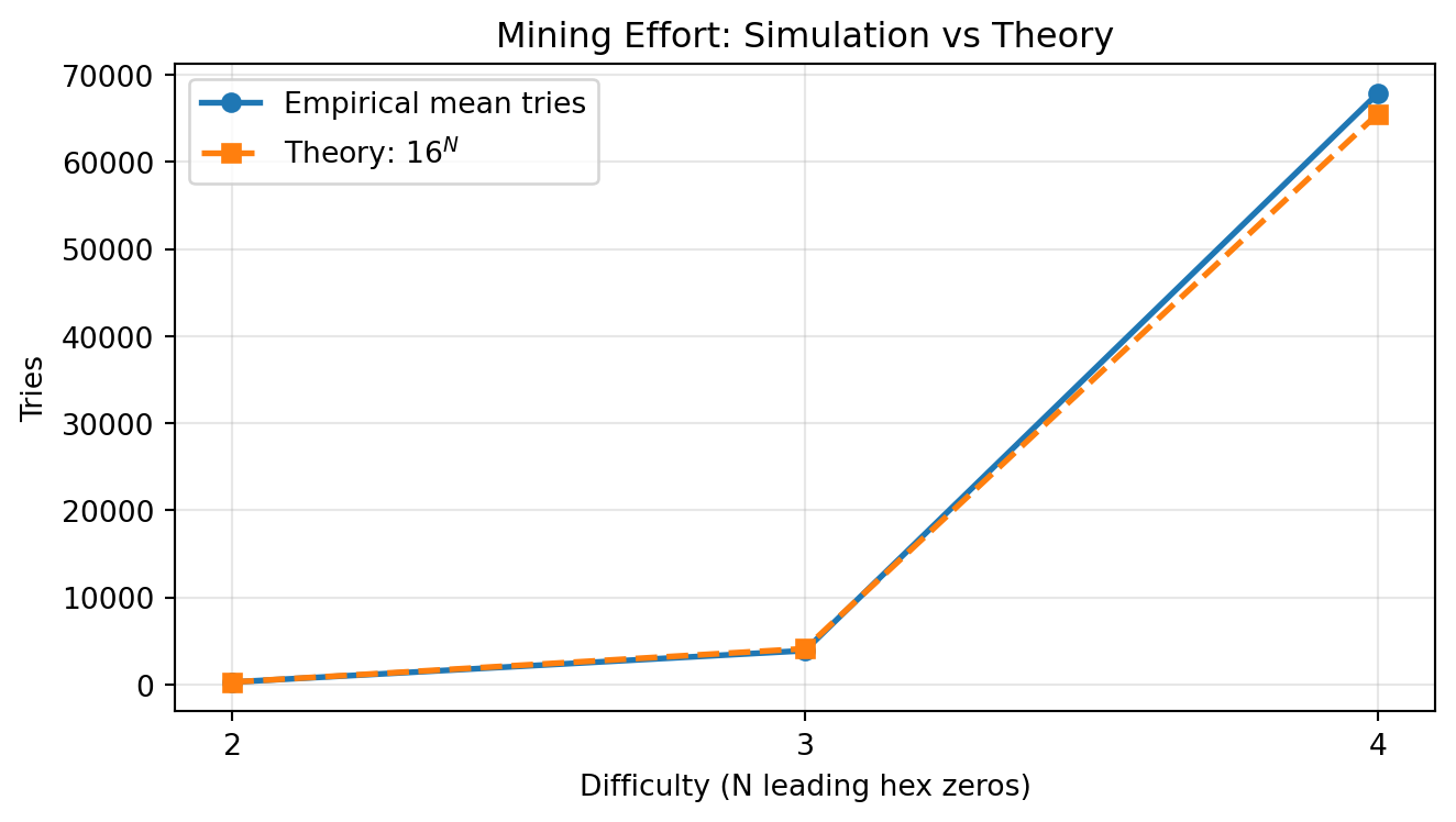
You can also inspect the dispersion in first-passage times for a fixed N. The distribution is right-skewed, so the mean is typically larger than the median.
N = 3
reps = 200
samples = [mine_once_leading_zeros(N) for _ in range(reps)]
df_dispersion = pd.DataFrame([{
"N": N,
"min": min(samples),
"median": statistics.median(samples),
"mean": round(statistics.mean(samples), 2),
"max": max(samples),
}])
df_dispersion| N | min | median | mean | max | |
|---|---|---|---|---|---|
| 0 | 3 | 115 | 2977.0 | 4005.36 | 19775 |
These simulations numerically recover the main PoW intuition: as difficulty increases by one more leading hex zero, expected mining effort scales by roughly a factor of 16.
These results empirically confirm the exponential scaling predicted by the geometric model. Even at modest difficulty (N=4), the expected number of hash attempts already reaches tens of thousands — illustrating why increasing difficulty rapidly raises the bar for successful mining and for rewriting history.
In the discrete deficit model, let Q_z be the probability an attacker eventually catches up when starting z blocks behind. The one-step recursion is Q_z = pQ_{z+1} + qQ_{z-1}, \quad z\ge 1, with boundary condition Q_0=1, where p is the honest-miner probability, q is attacker probability, and p+q=1.
Try a solution of the form Q_z=r^z. Substituting gives r^z = pr^{z+1}+qr^{z-1} \;\Longrightarrow\; pr^2-r+q=0. The roots are r=1 and r=q/p, so the general solution is Q_z = A + B\left(\frac{q}{p}\right)^z.
If p>q, we require \lim_{z\to\infty}Q_z=0 (the attacker has negative drift and catch-up chance vanishes from very deep deficits), so A=0. Using Q_0=1 then gives B=1, hence Q_z=\left(\frac{q}{p}\right)^z,\quad p>q. If p\le q, the attacker catches up with probability 1, so Q_z=1,\quad p\le q. Therefore, Q_z= \begin{cases} 1, & p \le q,\\ \left(\frac{q}{p}\right)^z, & p>q. \end{cases}
As an optional extension, we can embed the discrete deficit walk in a continuous-time diffusion (Brownian motion with drift). In the same model, with attacker deficit D_n and one-step moves +1 (probability p) or -1 (probability q), the exact catch-up probability from depth z is the formula above.
To see where the Brownian approximation comes from, start from one-step increments \Delta D = \begin{cases} +1,& \text{prob } p,\\ -1,& \text{prob } q. \end{cases} So \mathbb{E}[\Delta D]=p-q\equiv \mu,\qquad \mathrm{Var}(\Delta D)=4pq\equiv \sigma^2. Under diffusion scaling (many small steps over long horizons), D_n is approximated by dX_t=\mu\,dt+\sigma\,dW_t, with initial condition X_0=z.
Let u(x) be the probability that this diffusion ever hits 0 when starting from x>0. Standard generator arguments give \mu u'(x)+\frac{\sigma^2}{2}u''(x)=0, with boundary conditions u(0)=1,\qquad \lim_{x\to\infty}u(x)=0 \quad (\mu>0). Solving this ODE yields u(x)=\exp\!\left(-\frac{2\mu x}{\sigma^2}\right). Evaluating at x=z gives the Brownian catch-up approximation: Q_z^{\text{BM}} \approx \exp\!\left(-\frac{2\mu z}{\sigma^2}\right), \quad (\mu>0).
Substituting the random-walk moments, \mu = p-q,\qquad \sigma^2 = 4pq, gives Q_z^{\text{BM}} \approx \exp\!\left(-\frac{(p-q)z}{2pq}\right), \quad (p>q). Near the symmetric case (p \approx q), this is close to the first-order form \exp(-2(p-q)z).
import numpy as np
import matplotlib.pyplot as plt

def exact_ruin(q, z):
    p = 1 - q
    return 1.0 if p <= q else (q / p) ** z

def bm_approx(q, z):
    p = 1 - q
    if p <= q:
        return 1.0
    mu = p - q
    sigma2 = 4 * p * q
    return np.exp(-2 * mu * z / sigma2)

q = 0.30
z_values = np.arange(0, 21)

exact_vals = [exact_ruin(q, z) for z in z_values]
bm_vals = [bm_approx(q, z) for z in z_values]

plt.figure(figsize=(7, 4))
plt.plot(z_values, exact_vals, linewidth=2, label="Exact")
plt.plot(z_values, bm_vals, linestyle="--", linewidth=2, label="BM approx")
plt.xlabel("Confirmations z")
plt.ylabel("Catch-up probability")
plt.title(f"Catch-Up Probability: Exact vs BM Approximation (q = {q:.2f})")
plt.grid(alpha=0.3)
plt.legend()
plt.tight_layout()
plt.show()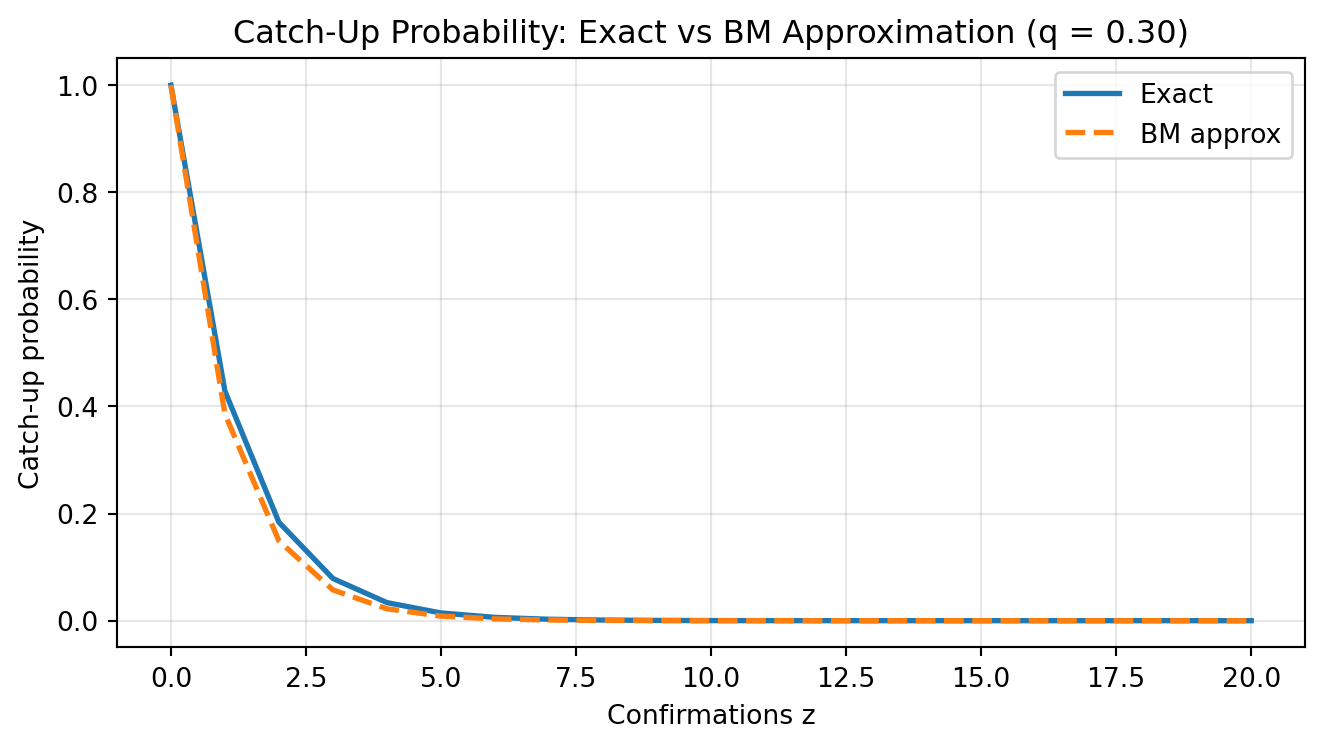
This appendix is mainly useful for readers with stochastic-process background. The main text should still rely on the exact discrete formula for interpretation.