import numpy as np
import pandas as pd
import matplotlib.pyplot as plt
import yfinance as yf
import seaborn as sns
import statsmodels.formula.api as smf

import warnings
warnings.simplefilter(action='ignore', category=FutureWarning)A Market Index for Cryptocurrencies
Introduction
In this notebook, we build a market index for cryptocurrencies. We then use this index to analyze the relationship between individual cryptocurrency returns and market-index returns. Finally, we analyze the relationship between crypto market returns and stock market returns.
Building a Crypto Market Index
The code below downloads data for the following cryptocurrencies:
| Ticker | Name |
|---|---|
| BTC | Bitcoin |
| ETH | Ethereum |
| BCH | Bitcoin Cash |
| LTC | Litecoin |
| XRP | Ripple |
| DOGE | Dogecoin |
| XLM | Stellar |
We include these seven coins because they have sufficiently long time series. The code also computes monthly returns and stores them in a DataFrame called df. This DataFrame has one column per coin and one row per month.
As always, we start by loading the required libraries. In this notebook, we use statsmodels to run linear regressions.
We now download cryptocurrency prices and compute returns. The code below downloads daily data, resamples to month-end observations, computes percentage returns, and drops missing values.
coins = ['BTC-USD','ETH-USD','LTC-USD','XRP-USD','DOGE-USD','BCH-USD','XLM-USD']

df = (
    yf.download(coins, start='2015-01-01', progress=False)['Close']
      .resample('ME')
      .last()
      .pct_change()
      .dropna()
)

df.columns = [c.replace('-USD','') for c in df.columns]
We will use the following weights to construct our crypto market index. For simplicity, the weights are constant over time. In practice, we could update them monthly based on market capitalization or use another weighting scheme. These weights are based on each coin’s market capitalization as of June 2024. Bitcoin (BTC) receives the largest weight, consistent with its much larger market capitalization.
w_raw = pd.Series({
    'BTC': 57.5,
    'ETH': 11.6,
    'XRP': 3.8,
    'DOGE': 0.7,
    'BCH': 0.4,
    'LTC': 0.2,
    'XLM': 0.2
})
Next, we build the crypto market index. We first normalize the weights so they sum to one, then expand them into a Pandas DataFrame with the same shape and index as the returns DataFrame. The variable mkt_ret is the weighted sum of cryptocurrency returns.
w = (w_raw / w_raw.sum())
weights = pd.DataFrame(np.tile(w.values, (len(df.index), 1)), index=df.index, columns=w.index)
mkt_ret = (weights * df).sum(axis=1)
df['MKT'] = mkt_ret
We can now plot the crypto market index. As the figure shows, it is highly volatile.
ax = df['MKT'].plot(title='Crypto Market Index')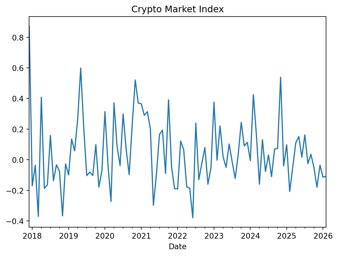
To better benchmark this volatility, we also download SPY returns and plot them with the crypto market index. This provides a direct comparison of crypto and stock market volatility. The code below downloads SPY data, resamples to month-end observations, computes returns, and drops missing values.
df['SPY'] = (yf
             .download('SPY', start='2015-01-01', progress=False)
             .loc[:,'Close']
             .resample('ME')
             .last()
             .pct_change()
             .dropna())
ax = df.loc[:,['MKT', 'SPY']].plot(title='Crypto Market Index and SPY')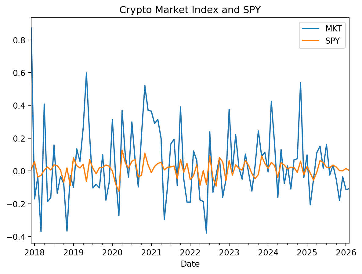
The previous figure shows that cryptocurrencies are much more volatile than stocks. The volatility of the crypto market index appears roughly three to four times higher than SPY’s volatility.
Analyzing the Relationship Between Cryptocurrencies and the Crypto Market Index
Returning to the main objective, we now examine how well the crypto market index explains individual coin returns. We should expect BTC to track the index closely. The scatter plot below compares BTC returns with market-index returns and shows a strong relationship, which is expected given BTC’s large index weight.
ax = sns.lmplot(data=df, x='MKT', y='BTC')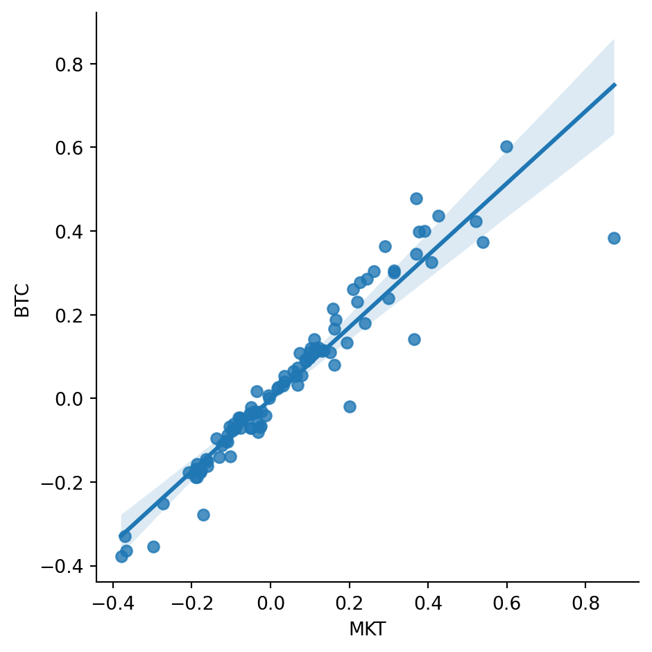
To formalize this relationship, we run the following regression with statsmodels:
r_{BTC} = \alpha + \beta r_{MKT} + e.
The code below runs the regression and prints the summary output, including coefficient estimates, standard errors, t-statistics, p-values, confidence intervals, and R-squared.
res = smf.ols('BTC ~ MKT', data=df).fit()
print(res.summary(slim=True))
OLS Regression Results
==============================================================================
Dep. Variable: BTC R-squared: 0.902
Model: OLS Adj. R-squared: 0.901
No. Observations: 99 F-statistic: 896.0
Covariance Type: nonrobust Prob (F-statistic): 8.63e-51
==============================================================================
coef std err t P>|t| [0.025 0.975]
------------------------------------------------------------------------------
Intercept -0.0023 0.006 -0.356 0.722 -0.015 0.010
MKT 0.8613 0.029 29.933 0.000 0.804 0.918
==============================================================================
Notes:
[1] Standard Errors assume that the covariance matrix of the errors is correctly specified.The regression reports several useful statistics. R-squared measures the share of return variance explained by the market index. Here, R-squared is high, as expected, because BTC is a large part of the index. The coefficient on MKT is the beta estimate and is slightly below one. Its p-value is very small, so we reject the null hypothesis that beta is zero. In other words, BTC returns are strongly and statistically significantly related to market-index returns.
Now let’s analyze a coin with a smaller index weight: BCH. The scatter plot below shows BCH versus MKT, with noticeably more dispersion than BTC.
ax = sns.lmplot(data=df, x='MKT', y='BCH')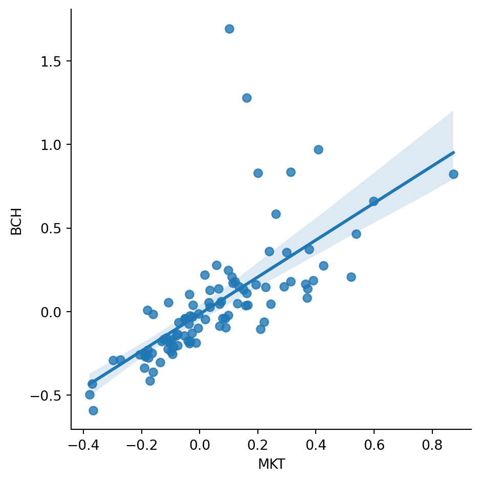
The BCH regression shows a beta slightly above one, but a lower R-squared.
res = smf.ols('BCH ~ MKT', data=df).fit()
print(res.summary(slim=True))
OLS Regression Results
==============================================================================
Dep. Variable: BCH R-squared: 0.474
Model: OLS Adj. R-squared: 0.469
No. Observations: 99 F-statistic: 87.57
Covariance Type: nonrobust Prob (F-statistic): 3.26e-15
==============================================================================
coef std err t P>|t| [0.025 0.975]
------------------------------------------------------------------------------
Intercept -0.0131 0.026 -0.496 0.621 -0.065 0.039
MKT 1.1012 0.118 9.358 0.000 0.868 1.335
==============================================================================
Notes:
[1] Standard Errors assume that the covariance matrix of the errors is correctly specified.We can use a for loop to estimate all betas and R-squared values at once. The code below regresses each coin on the crypto market index and stores the outputs in a DataFrame. Notice that the MKT row is an intentional sanity check: regressing MKT on itself gives a beta of 1 and an R-squared of 1.
results = []
for c in df.columns:
    if c == 'SPY':
        continue
    res = smf.ols(f'{c} ~ MKT', data=df).fit()
    results.append({
        'Coin': c,
        'Beta': res.params['MKT'],
        'R-squared': res.rsquared
    })

results_df = pd.DataFrame(results)
results_df['Beta'] = results_df['Beta'].round(2)
results_df['R-squared'] = results_df['R-squared'].round(3)
display(results_df)| Coin | Beta | R-squared | |
|---|---|---|---|
| 0 | BCH | 1.10 | 0.474 |
| 1 | BTC | 0.86 | 0.902 |
| 2 | DOGE | 2.13 | 0.229 |
| 3 | ETH | 1.08 | 0.721 |
| 4 | LTC | 1.06 | 0.689 |
| 5 | XLM | 2.07 | 0.433 |
| 6 | XRP | 2.59 | 0.368 |
| 7 | MKT | 1.00 | 1.000 |
Interestingly, Dogecoin (DOGE), Stellar (XLM), and Ripple (XRP) have relatively high betas, meaning their returns are quite sensitive to the market index on average. However, their R-squared values are low, indicating that the index explains only a limited share of their return variation. This pattern suggests substantial coin-specific risk, or variation not captured by the market factor. In crypto markets, that could reflect factors such as technology, governance, adoption, or specific use cases.
Crypto Market Index vs. Stock Market
Finally, we can explore how well the stock market explains variation in crypto market returns. The graph below suggests that a large share of crypto return variance is not explained by the stock market, which points to potential diversification benefits.
ax = sns.lmplot(data=df, x='SPY', y='MKT')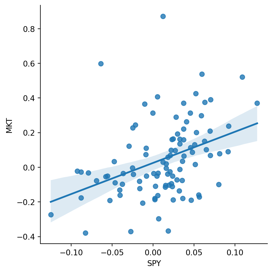
A regression of crypto market returns on the stock market portfolio suggests a beta around 1.8. The coefficient p-value is very small, so we reject the null hypothesis that beta is zero.
res = smf.ols('MKT ~ SPY', data=df).fit()
print(res.summary(slim=True))
OLS Regression Results
==============================================================================
Dep. Variable: MKT R-squared: 0.148
Model: OLS Adj. R-squared: 0.139
No. Observations: 99 F-statistic: 16.81
Covariance Type: nonrobust Prob (F-statistic): 8.59e-05
==============================================================================
coef std err t P>|t| [0.025 0.975]
------------------------------------------------------------------------------
Intercept 0.0249 0.021 1.176 0.242 -0.017 0.067
SPY 1.8052 0.440 4.100 0.000 0.931 2.679
==============================================================================
Notes:
[1] Standard Errors assume that the covariance matrix of the errors is correctly specified.We can also test whether the coefficient differs from 1. The F-test p-value is 0.07, so at the 5% level we fail to reject the null hypothesis that the coefficient equals 1.
hypothesis = 'SPY = 1'
f_test = res.f_test(hypothesis)
print(f"F-statistic: {f_test.fvalue:.4f}")
print(f"P-value: {f_test.pvalue:.4f}")
print(f"Degrees of freedom (numerator, denominator): {f_test.df_num}, {f_test.df_denom}")
F-statistic: 3.3445
P-value: 0.0705
Degrees of freedom (numerator, denominator): 1.0, 97.0