Introduction to Jupyter Notebooks

The objective of this class was to quickly introduce to Python students who have never used it before, and to show some interesting financial applications.

Libraries

We started loading some of the typical libraries that we will use in the class.

import numpy as np
import pandas as pd
import matplotlib.pyplot as plt
import yfinance as yf
import seaborn as sns

import warnings
warnings.simplefilter(action='ignore', category=FutureWarning)

A very useful library for finance applications is yfinance. This library allows us to download data from Yahoo Finance and use it to perform analyses on stock prices for example.

The library yfinance downloads the data as a Pandas dataframe. If we want then to use Pandas functions on the dataframe then we need to load the library pandas. Each pandas dataframe allows us to plot its content. To plot something else, we need the library matplotlib. The library seaborn is just a nice plotting library that has additional feature.

Since yfinance has had many changes recently, you typically get some warnings that I disable using the warnings library.

As an example of using yfinance, let’s compute the monthly rate of return of Microsoft (MSFT) and an ETF on the S&P 500 (SPY).

df = (yf
      .download(['MSFT', 'SPY'], progress=False, start='2000-01-01')
      .loc[:,'Close']
      .resample('ME')
      .last()
      .pct_change()
      )

The code above uses yfinance to download data for ['MSFT', 'SPY'] starting in January 1, 2000. It then extracts the Close column, which is adjusted close data by default in yfinance. The resulting pandas dataframe is resampled monthly, and pct_change computes the required returns.

We can now plot the monthly returns of MSFT and SPY.

ax = df.plot(title = 'Monthly Returns of MSFT Stock and SPY')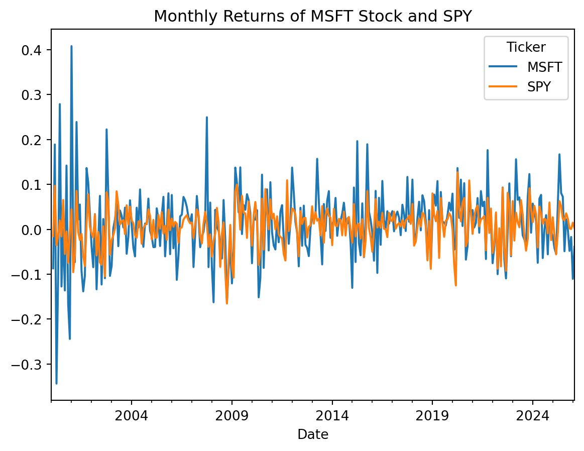

We can clearly see from the picture that the returns of the SPY are less volatile than the returns on MSFT. This makes sense, as the SPY is a well diversified portfolio of stocks whereas MSFT is a single name stock.

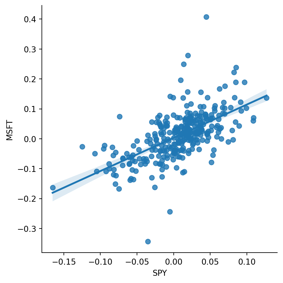
There is, however, a strong co-movement between the returns of MSFT and SPY. To see this, we could regress the monthly MSFT returns on the monthly SPY returns as: R_{MSFT} = \alpha + \beta R_{SPY} + e. The graph below shows the result of this regression.

ax = sns.lmplot(df, x = 'SPY', y = 'MSFT')