import numpy as np
import pandas as pd
import matplotlib.pyplot as plt
from scipy.optimize import minimize
import yfinance as yf

import warnings
warnings.simplefilter(action='ignore', category=FutureWarning)Minimum Variance Portfolio
Introduction
This notebook estimates a minimum variance equity portfolio using monthly returns and compares two versions of the optimizer:
No Short: weights constrained to lie between 0 and 1.Short Allowed: weights can be negative.
I estimate weights on data from January 2020 to December 2024, then evaluate out-of-sample performance from January 2025 onward against SPY.
Setup
I import the libraries needed for data handling, optimization, and plotting. I also suppress a Yahoo Finance warning so notebook output stays clean.
Build the Universe and Returns Panel
I start from a market-cap file as of December 2024 and define key dates/parameters up front. You can download the market cap file from this link. Remember to place it in the same folder as this notebook.
TRAIN_END = '2024-12-31'
TEST_START = '2025-01-01'
MIN_MONTHS = 36
N_TOP = 50

mcap = pd.read_csv('stocks_mktcap_202412.csv')
tickers = mcap['TICKER'].unique().tolist()
I then download adjusted close prices, convert to month-end returns, and keep the full panel before applying train/test-specific missing-data rules.
rets = (yf
      .download(tickers, start='2020-01-01', progress=False)['Close']
      .resample('ME')
      .last()
      .pct_change()
      .dropna(how='all')
      )
To avoid look-ahead bias, I apply the data-availability filter using only the training window. Then I keep the largest N_TOP eligible stocks by market cap.
train_rets = rets.loc[:TRAIN_END]

valid = train_rets.count() >= MIN_MONTHS
eligible = mcap.loc[mcap['TICKER'].isin(train_rets.columns[valid])]

top = (
    eligible.sort_values('MCAP', ascending=False)
            .head(N_TOP)['TICKER']
            .tolist()
)

df = rets[top]
train = df.loc[:TRAIN_END]
test = df.loc[TEST_START:].dropna()
Estimate Minimum Variance Weights
For weights vector \mathbb{w} and covariance matrix \Sigma, portfolio variance is \sigma_P^2 = \mathbb{w}' \Sigma \mathbb{w}, with budget constraint \sum_{i = 1}^n w_i = \mathbb{w}' \boldsymbol{\iota} = 1.
I solve this with SLSQP once with bounds (No Short) and once without bounds (Short Allowed).
n = train.shape[1]
cov = train.cov().values
w0 = np.ones(n) / n
objective = lambda w: w @ cov @ w
sum_to_one = {'type': 'eq', 'fun': lambda w: w.sum() - 1}

res = minimize(
    objective,
    w0,
    method='SLSQP',
    bounds=[(0, 1)] * n,
    constraints=[sum_to_one]
)

res_short = minimize(
    objective,
    w0,
    method='SLSQP',
    constraints=[sum_to_one]
)

if (not res.success) or (not res_short.success):
    raise RuntimeError(
        f"Optimization failed: no-short={res.message}; short-allowed={res_short.message}"
    )
Inspect Estimated Weights
The first plot shows the no-short solution. Because weights are constrained to be nonnegative, several stocks receive zero weight.
min_display_weight = 0.005

weights = (
    pd.DataFrame({'TICKER': train.columns, 'WEIGHT': res.x})
      .query('WEIGHT > @min_display_weight')
      .sort_values('WEIGHT', ascending=False)
)

plt.figure()
plt.barh(weights['TICKER'], weights['WEIGHT'])
plt.gca().invert_yaxis()
plt.title('Minimum Variance Portfolio Weights (No Short)')
plt.xlabel('Weight')
plt.tight_layout()
plt.show()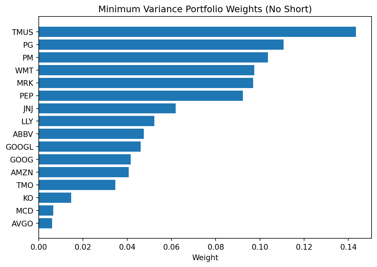
The second plot shows the short-allowed solution. Positive weights are long positions and negative weights are short positions.
weights_short = (
    pd.DataFrame({'TICKER': train.columns, 'WEIGHT': res_short.x})
      .query('abs(WEIGHT) > @min_display_weight')
      .sort_values('WEIGHT', ascending=False)
)

colors = np.where(weights_short['WEIGHT'] >= 0, 'tab:blue', 'tab:red')

plt.figure()
plt.barh(weights_short['TICKER'], weights_short['WEIGHT'], color=colors)
plt.axvline(0, color='black', linewidth=0.8)
plt.gca().invert_yaxis()
plt.title('Minimum Variance Portfolio Weights (Short Allowed)')
plt.xlabel('Weight')
plt.tight_layout()
plt.show()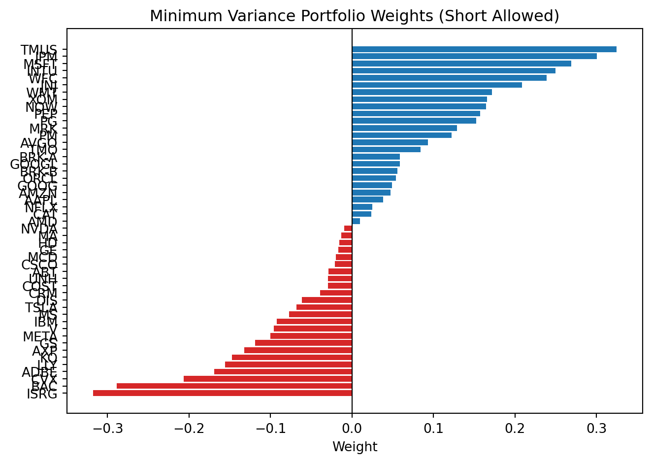
When short sales are allowed, weights are typically more extreme because the optimizer can offset exposures with negative positions.
Backtest: January 2025 Onward
Next I compute out-of-sample monthly returns for both portfolios:
No Short: minimum variance with weights constrained to be between 0 and 1.Short Allowed: minimum variance with no bounds on individual weights.
w_noshort = res.x
w_short = res_short.x

port_rets_noshort = test @ w_noshort
port_rets_short = test @ w_short
I compare both series with SPY over the same months.
spy = (
    yf.download('SPY', start=TEST_START, progress=False)['Close']
      .resample('ME')
      .last()
      .pct_change()
)

spy_test = spy.loc[TEST_START:].squeeze()
I align all series to common dates and compute cumulative returns.
aligned = pd.concat(
    [
        port_rets_noshort.rename('No Short'),
        port_rets_short.rename('Short Allowed'),
        spy_test.rename('SPY')
    ],
    axis=1
).dropna()

cum_noshort = (1 + aligned['No Short']).cumprod()
cum_short = (1 + aligned['Short Allowed']).cumprod()
cum_spy = (1 + aligned['SPY']).cumprod()
The plot below compares cumulative performance.
plt.figure()
plt.plot(cum_noshort, label='No Short')
plt.plot(cum_short, label='Short Allowed')
plt.plot(cum_spy, label='SPY')
plt.legend()
plt.title('Cumulative Returns: No-Short vs Short-Allowed')
plt.show()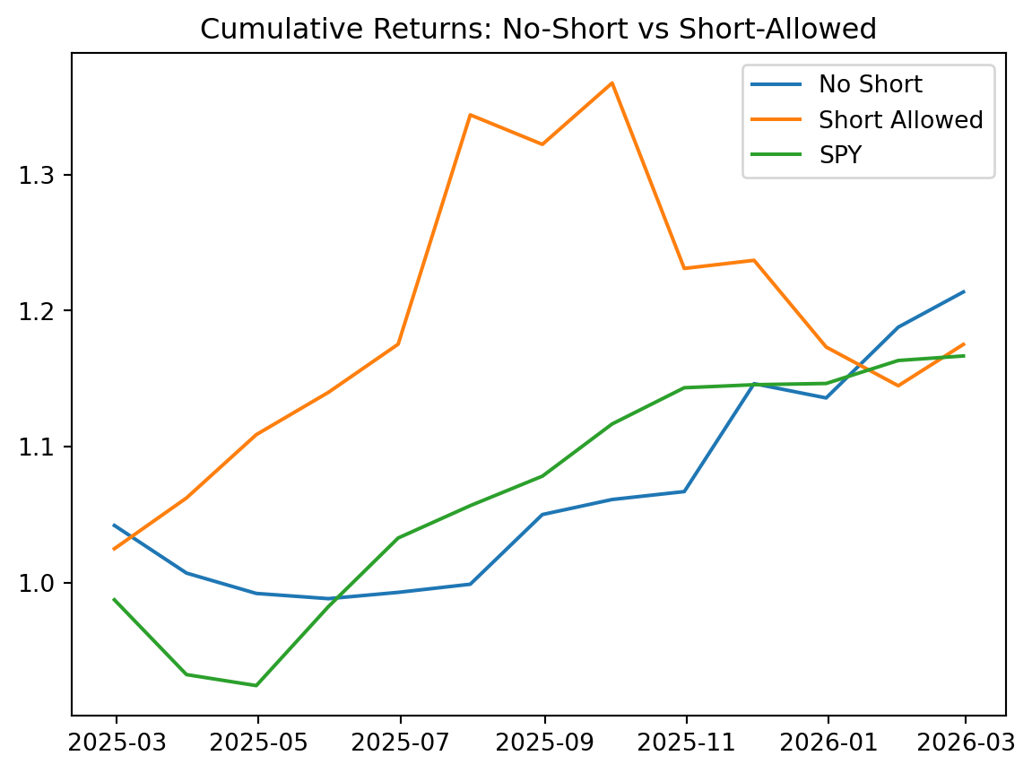
In this sample, the No Short portfolio performs better than both Short Allowed and SPY. This is consistent with Jagannathan and Ma (2003): in large portfolios, no-short constraints can reduce the impact of covariance estimation error by shrinking extreme positions.
Jagannathan, Ravi, and Tongshu Ma. 2003. “Risk Reduction in Large Portfolios: Why Imposing the Wrong Constraints Helps.” Journal of Finance 58 (4): 1651–83.
Note that the idea of this portfolio is to improve the Sharpe ratio by reducing volatility, not to generate an alpha. In fact, the expected return of the minimum variance portfolio is typically lower than that of the market. The goal is to achieve a better risk-adjusted return by reducing volatility, even if it means accepting a lower expected return.
Also note that when short-selling is allowed, the optimizer can take on large positive and negative positions that may not be realistic in practice due to transaction costs, liquidity constraints, or risk management policies. The no-short solution is often more stable and easier to implement, especially for individual investors or funds with limited resources.