start_date = "1994-12-01"
end_date = "2026-01-01"
ticker = "FDVLX"Analyzing Mutual Fund Performance
Mutual Funds
One of the main uses of asset pricing models is to analyze the performance of mutual funds. A mutual fund is a type of investment vehicle that pools money from many individual investors to purchase a diversified portfolio of stocks, bonds, or other securities. The fund is managed by a professional portfolio manager who invests the money in accordance with the fund’s investment objectives and strategy.
There are many different types of mutual funds, including equity funds, bond funds, balanced funds, index funds, and specialty funds. Each type of fund has its own investment strategy and risk profile, and investors should carefully consider their investment objectives and risk tolerance before choosing a mutual fund to invest in.
In this notebook I analyze the Fidelity Value Fund (Ticker: FDVLX). According to the fund description, the fund invests in securities of companies that possess valuable fixed assets or that the fund manager believes are undervalued in the marketplace in relation to factors such as assets, earnings, or growth potential (stocks of these companies are often called “value” stocks). Normally investing primarily in common stocks.
The Augmented Five-Factor Model
We will estimate the Fama-French five-factor model augmented by the momentum factor, R_{i} = a_{i} + b_{i} R_{m} + s_{i} \mathit{SMB} + h_{i} \mathit{HML} + r_{i} \mathit{RMW} + c_{i} \mathit{CMA} + m_{i} \mathit{MOM} + e_{i} where R_{i} = r_{i} - r_{f} represents the monthly excess returns for security i over the risk-free rate, and R_{m} = r_{m} - r_{f} represents the monthly excess returns of the market.
The estimation of a_{i}, which is commonly called the alpha, now controls for many important sources of variation in the investment opportunity set. If the model is correct then the alpha should be close to zero.
The different loadings on the factors also have a clear interpretation. For a mutual fund we have that:
- b_{i} < 1 implies that the fund has less systematic risk than the market whereas a b_{i} > 1 implies that the fund takes more systematic risk than the market.
- s_{i} > 0 implies that the fund loads mostly on small stocks whereas s_{i} < 0 implies that the fund loads on large stocks.
- h_{i} > 0 implies that the fund loads on value stocks whereas h_{i} < 0 implies that the fund loads on growth stocks.
- r_{i} > 0 implies that the fund loads on stocks with robust operating profitability whereas r_{i} < 0 implies that the fund loads on stocks with weak operating profitability.
- c_{i} > 0 implies that the fund loads on stocks with low investment whereas c_{i} < 0 implies that the fund loads on stocks with high investments.
- m_{i} > 0 implies that the fund loads on winners whereas a negative m_{i} < 0 implies that the fund loads on losers, i.e. follows a contrarian strategy.
The Capital Asset Pricing Model (CAPM) is obtained by restricting s_{i} = 0, h_{i} = 0, r_{i} = 0, c_{i} = 0, and m_{i} = 0. Other nested models such as the Fama-French three-factor model can be obtained in a similar way.
Python Packages
import pandas as pd
import getfactormodels as gfm
import yfinance as yf
import statsmodels.formula.api as smf
import matplotlib.pyplot as plt

import warnings
warnings.simplefilter(action="ignore", category=FutureWarning)
Getting the Factors
The following code downloads the factors from the Fama-French five-factor model augmented by the momentum factor. I used to download this data using pandasdatareader, but the library is no longer maintained and does not work with Python 3.14. Thus, I switched to getfactormodels, which works very well.
ff5 = gfm.FamaFrenchFactors(model="5", frequency="m").to_pandas()
carhart = gfm.CarhartFactors(frequency="m").to_pandas()

ff_mom = pd.merge(ff5, carhart[['MOM']], left_index=True, right_index=True)
ff_mom = ff_mom.rename(columns={"Mkt-RF": "RMRF"})

ff_mom.index = pd.to_datetime(ff_mom.index)

display(ff_mom)| RMRF | SMB | HML | RMW | CMA | RF | MOM | |
|---|---|---|---|---|---|---|---|
| date | |||||||
| 1963-07-31 | -0.0039 | -0.0048 | -0.0081 | 0.0064 | -0.0115 | 0.0027 | 0.0101 |
| 1963-08-31 | 0.0508 | -0.0080 | 0.0170 | 0.0040 | -0.0038 | 0.0025 | 0.0100 |
| 1963-09-30 | -0.0157 | -0.0043 | 0.0000 | -0.0078 | 0.0015 | 0.0027 | 0.0012 |
| 1963-10-31 | 0.0254 | -0.0134 | -0.0004 | 0.0279 | -0.0225 | 0.0029 | 0.0313 |
| 1963-11-30 | -0.0086 | -0.0085 | 0.0173 | -0.0043 | 0.0227 | 0.0027 | -0.0078 |
| ... | ... | ... | ... | ... | ... | ... | ... |
| 2025-08-31 | 0.0185 | 0.0488 | 0.0442 | -0.0068 | 0.0208 | 0.0038 | -0.0354 |
| 2025-09-30 | 0.0339 | -0.0218 | -0.0105 | -0.0206 | -0.0222 | 0.0033 | 0.0463 |
| 2025-10-31 | 0.0196 | -0.0131 | -0.0309 | -0.0521 | -0.0403 | 0.0037 | 0.0027 |
| 2025-11-30 | -0.0013 | 0.0147 | 0.0376 | 0.0142 | 0.0068 | 0.0030 | -0.0180 |
| 2025-12-31 | -0.0036 | -0.0022 | 0.0242 | 0.0040 | 0.0037 | 0.0034 | -0.0241 |
750 rows × 7 columns
Getting the Data Ready
Fund Returns
We download the close price series from Yahoo! Finance. For mutual funds the close and adjusted close price is the same since for tax purposes mutual funds reinvest all dividend payments in the fund.
stock = yf.download(tickers=ticker, start=start_date, end=end_date, progress=False, multi_level_index=False).loc[:, ['Close']]
ax = stock.plot(title="Price of " + ticker)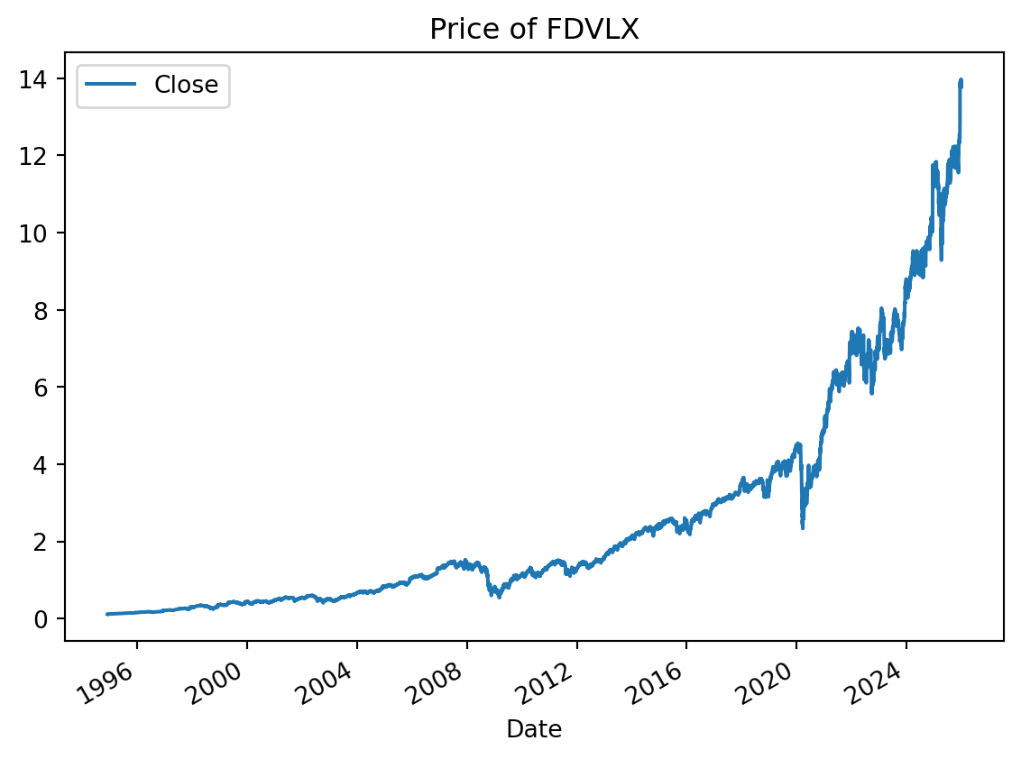
We compute monthly returns and use RET to denote the column containing the returns.
ret = stock.resample("ME").last().pct_change()
ret = ret.rename(columns={"Close": "RET"})
ax = ret.plot(title="Monthly Return on " + ticker)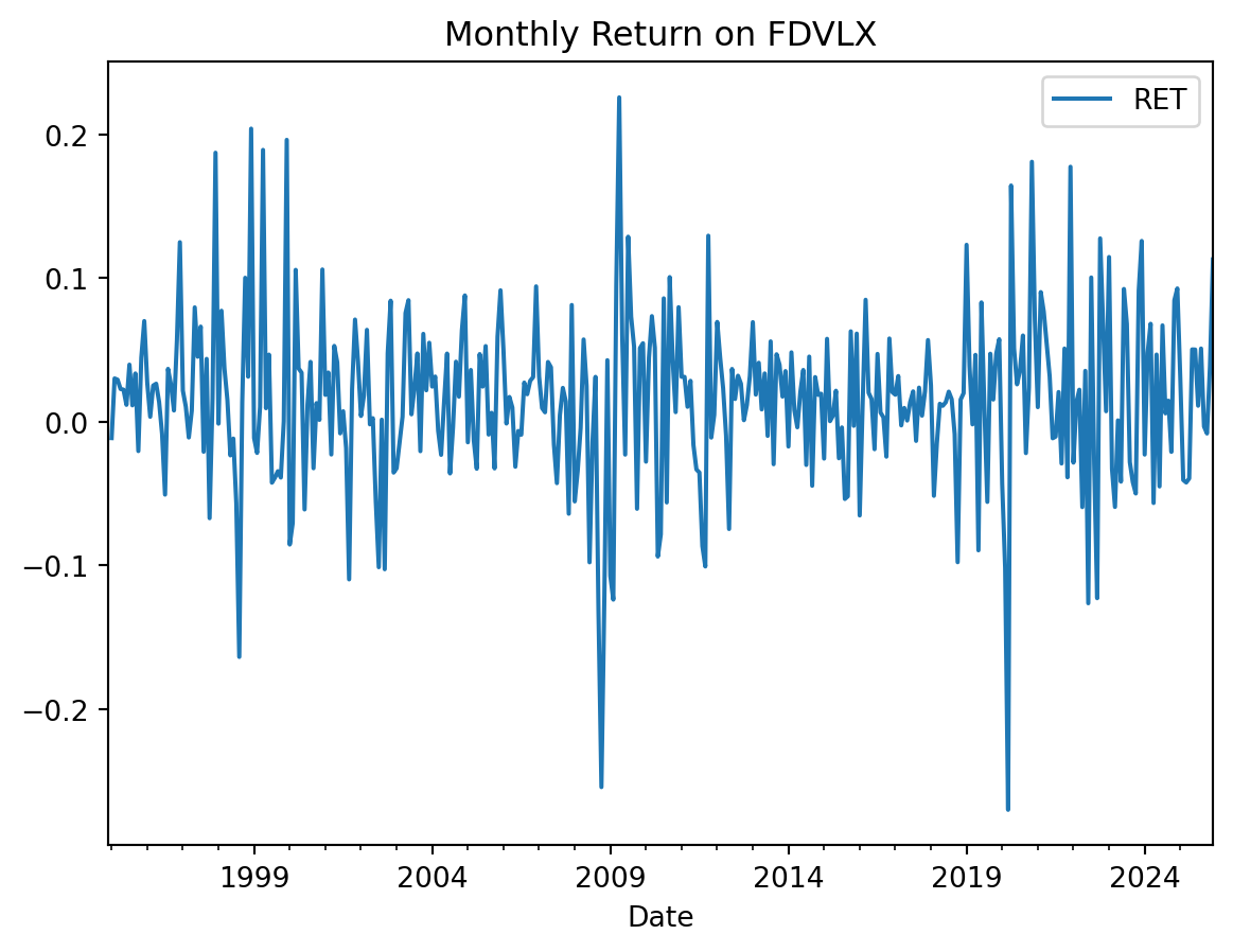
Merge with the Factors
Finally, we merge the returns series that we want to analyze with the six factors. Additionally, we compute excess returns for the security.
merged = (
    pd.merge(left=ret, right=ff_mom, left_index=True, right_index=True)
    .assign(RETRF=ret["RET"] - ff_mom["RF"])
    .drop(columns=["RET", "RF"])
    .dropna()
)
display(merged)| RMRF | SMB | HML | RMW | CMA | MOM | RETRF | |
|---|---|---|---|---|---|---|---|
| Date | |||||||
| 1995-01-31 | 0.0180 | -0.0307 | 0.0259 | 0.0015 | -0.0065 | -0.0184 | -0.015717 |
| 1995-02-28 | 0.0363 | -0.0049 | 0.0099 | 0.0061 | -0.0040 | -0.0047 | 0.025995 |
| 1995-03-31 | 0.0219 | -0.0053 | -0.0213 | -0.0013 | 0.0023 | 0.0045 | 0.024522 |
| 1995-04-30 | 0.0211 | -0.0026 | 0.0167 | 0.0043 | 0.0082 | 0.0180 | 0.018285 |
| 1995-05-31 | 0.0290 | -0.0217 | 0.0228 | 0.0041 | 0.0001 | -0.0055 | 0.016782 |
| ... | ... | ... | ... | ... | ... | ... | ... |
| 2025-08-31 | 0.0185 | 0.0488 | 0.0442 | -0.0068 | 0.0208 | -0.0354 | 0.046998 |
| 2025-09-30 | 0.0339 | -0.0218 | -0.0105 | -0.0206 | -0.0222 | 0.0463 | -0.006753 |
| 2025-10-31 | 0.0196 | -0.0131 | -0.0309 | -0.0521 | -0.0403 | 0.0027 | -0.012016 |
| 2025-11-30 | -0.0013 | 0.0147 | 0.0376 | 0.0142 | 0.0068 | -0.0180 | 0.035435 |
| 2025-12-31 | -0.0036 | -0.0022 | 0.0242 | 0.0040 | 0.0037 | -0.0241 | 0.109415 |
372 rows × 7 columns
Estimating the Model
CAPM
We start by estimating a CAPM regression, R_{i} = a_{i} + b_{i} R_{m} + e_{i}
results = smf.ols("RETRF ~ RMRF", data=merged).fit()
print(results.summary(slim=True))
OLS Regression Results
==============================================================================
Dep. Variable: RETRF R-squared: 0.632
Model: OLS Adj. R-squared: 0.631
No. Observations: 372 F-statistic: 634.4
Covariance Type: nonrobust Prob (F-statistic): 3.03e-82
==============================================================================
coef std err t P>|t| [0.025 0.975]
------------------------------------------------------------------------------
Intercept 0.0043 0.002 2.282 0.023 0.001 0.008
RMRF 1.0445 0.041 25.187 0.000 0.963 1.126
==============================================================================
Notes:
[1] Standard Errors assume that the covariance matrix of the errors is correctly specified.The results indicate that the CAPM alpha is positive (a = 0.0043) and statistically significant at the 5% level (p-value = 0.023). This means that during the period the fund outperformed the market.
The Augmented Five-Factor Model
results = smf.ols("RETRF ~ RMRF + SMB + HML + RMW + CMA + MOM", data=merged).fit()
print(results.summary(slim=True))
OLS Regression Results
==============================================================================
Dep. Variable: RETRF R-squared: 0.760
Model: OLS Adj. R-squared: 0.756
No. Observations: 372 F-statistic: 192.4
Covariance Type: nonrobust Prob (F-statistic): 9.25e-110
==============================================================================
coef std err t P>|t| [0.025 0.975]
------------------------------------------------------------------------------
Intercept 0.0027 0.002 1.680 0.094 -0.000 0.006
RMRF 1.0648 0.039 26.989 0.000 0.987 1.142
SMB 0.3163 0.056 5.654 0.000 0.206 0.426
HML 0.3767 0.066 5.691 0.000 0.247 0.507
RMW 0.2921 0.071 4.106 0.000 0.152 0.432
CMA 0.1150 0.094 1.223 0.222 -0.070 0.300
MOM -0.1049 0.034 -3.062 0.002 -0.172 -0.038
==============================================================================
Notes:
[1] Standard Errors assume that the covariance matrix of the errors is correctly specified.After controlling for the other factors, the alpha is positive (a = 0.0027) but only marginally significant at the 10% level (p-value = 0.094). In other words, after controlling for our systematic factors the fund outperformed by 0.27 \times 12 = 3.24\% per year, though this result is not statistically significant at conventional levels.
We learn the following from the coefficient estimates.
| Factor | Coefficient | Significance | Interpretation |
|---|---|---|---|
| SMB | 0.3163 | 1% | The fund invested in small stocks |
| HML | 0.3767 | 1% | The fund invested in value stocks |
| RMW | 0.2921 | 1% | The fund invested in stocks with strong profitability |
| CMA | 0.1150 | Not significant | The fund invested in both high and low investment stocks |
| MOM | -0.1049 | 1% | The fund was significantly contrarian by chasing losers |
Therefore, the results from the regression somewhat agree with the fund description. The exposure to SMB is positive on size, even though Morningstar categorizes the fund as Mid-Cap Value. The fund returns load significantly on HML, which is consistent with the fund being a value fund. The negative exposure to momentum might come from the fact that value firms often have low P/E ratios, which commonly occur after stock price declines.