import numpy as np
import matplotlib.pyplot as plt

import torch
import torch.nn as nn
from torch.utils.data import DataLoader, TensorDataset

from scipy.stats import norm, binned_statistic

from sklearn.model_selection import train_test_split
from sklearn.preprocessing import StandardScalerOption Pricing with Neural Networks
Introduction
In this notebook, I implement a neural network to approximate the Black–Scholes option pricing formula. I generate synthetic data based on the Black–Scholes model, train a neural network on this data, and evaluate its performance. Finally, I visualize the prediction errors with respect to moneyness.
The Black-Scholes Model
The Black–Scholes model provides a theoretical framework for pricing European-style options. Remember that a European call option gives the holder the right, but not the obligation, to buy an underlying asset at a specified strike price K on a specified expiration date T. In the following, S denotes the current stock price, r the risk-free interest rate, \sigma the volatility of the underlying asset, and N(\cdot) the cumulative distribution function of the standard normal distribution.
The formula for the price of a European call option is given by: C = S N(d_1) - K e^{-rT} N(d_2), where \begin{aligned} d_1 &= \frac{\ln(S / K) + (r + \frac{1}{2} \sigma^2) T}{\sigma \sqrt{T}}, \\ d_2 &= d_1 - \sigma \sqrt{T}. \end{aligned}
The Black-Scholes formula is consistent with the absence of arbitrage opportunities in efficient markets and assumes that the underlying asset follows a geometric Brownian motion with constant volatility and interest rates. Even though these assumptions may not hold perfectly in real markets, we will see if we can teach a neural network to approximate this formula.
Neural Networks
A neural network is a flexible function approximator built by composing linear maps and nonlinear activations. It is well suited to learning nonlinear relationships such as the mapping from option inputs to option prices.
For each option observation i, define the feature vector \mathbf{x}_i = \begin{pmatrix} S_i \\ r_i \\ T_i \\ \sigma_i \end{pmatrix}, \quad y_i = C_i, where y_i is the Black-Scholes call price. A feedforward network predicts \hat{y}_i = f(\mathbf{x}_i; \theta), with parameters \theta (all weights and biases). Training chooses \theta to make \hat{y}_i close to y_i.
For one hidden layer, a standard notation is \hat{y}_i = W^{(2)} \phi\left(W^{(1)} \mathbf{x}_i + b^{(1)}\right) + b^{(2)}, where \phi(\cdot) is the activation function. (We use \phi here so it is not confused with volatility \sigma.) When its input is a vector z \in \mathbb{R}^m, \phi(z) is understood elementwise: \phi(z)=\begin{pmatrix}\phi(z_1)&\cdots&\phi(z_m)\end{pmatrix}^{\top}\in\mathbb{R}^m. If the input dimension is d_x=4 and the hidden layer has size h, then W^{(1)} \in \mathbb{R}^{h \times d_x}, \quad b^{(1)} \in \mathbb{R}^{h}, \quad W^{(2)} \in \mathbb{R}^{1 \times h}, \quad b^{(2)} \in \mathbb{R}.
A typical activation function used in neural networks is the Rectified Linear Unit (ReLU), defined as: \text{ReLU}(x) = \max(0, x).
A network with two hidden layers can be written as: \hat{y}_i = W^{(3)} \phi\left(W^{(2)} \phi\left(W^{(1)} \mathbf{x}_i + b^{(1)}\right) + b^{(2)}\right) + b^{(3)}. With hidden sizes h_1 and h_2, the dimensions are W^{(1)} \in \mathbb{R}^{h_1 \times d_x}, \quad b^{(1)} \in \mathbb{R}^{h_1}, \quad W^{(2)} \in \mathbb{R}^{h_2 \times h_1}, \quad b^{(2)} \in \mathbb{R}^{h_2}, \quad W^{(3)} \in \mathbb{R}^{1 \times h_2}, \quad b^{(3)} \in \mathbb{R}. This recursive structure is the key idea: each layer transforms the previous layer’s output, and adding layers increases the model’s capacity to approximate complex functions such as Black-Scholes prices.
The training process involves adjusting the parameters \theta to minimize a loss function, such as Mean Squared Error (MSE), which measures the average squared difference between the predicted and true option prices: \text{MSE} = \frac{1}{N} \sum_{i=1}^{N} (\hat{y}_i - y_i)^2, where N is the number of training samples. Optimization algorithms like Stochastic Gradient Descent (SGD) or Adam are commonly used to update the parameters based on the gradients of the loss function with respect to the parameters.
It is usually good practice to train the neural network on a training dataset and evaluate its performance on a separate testing dataset to ensure that the model generalizes well to unseen data.
Generating the Training Data
We use PyTorch to build and train the neural network, and scikit-learn for preprocessing and train/test splitting.
We first set a random seed for reproducibility and choose the compute device.
seed = 420
np.random.seed(seed)
torch.manual_seed(seed)

device = torch.device("cuda" if torch.cuda.is_available() else "cpu")
print(f"Using device: {device}")
Using device: cudaFor this notebook, CPU training is typically sufficient because the dataset and model are small. A GPU becomes more important for larger datasets and deeper models.
Next, we define a vectorized Black-Scholes call-pricing function.
def bs_call(S, K, r, T, vol, eps=1e-12):
    S = np.asarray(S, dtype=float)
    K = np.asarray(K, dtype=float)
    r = np.asarray(r, dtype=float)
    T = np.maximum(np.asarray(T, dtype=float), eps)
    vol = np.maximum(np.asarray(vol, dtype=float), eps)

    d1 = (np.log(S / K) + (r + 0.5 * vol**2) * T) / (vol * np.sqrt(T))
    d2 = d1 - vol * np.sqrt(T)
    return S * norm.cdf(d1) - K * np.exp(-r * T) * norm.cdf(d2)
We now generate synthetic data on a grid of (S, r, T, \sigma) values, keep K=1, and create targets using Black-Scholes prices with small volatility noise.
S = np.arange(0.6, 1.4, 0.005)
r = np.arange(0.00, 0.06, 0.01)
T = np.arange(3/12, 2 + 1/12, 1/12)
vol = np.arange(0.1, 0.9, 0.1)

Sg, rg, Tg, vg = np.meshgrid(S, r, T, vol, indexing="ij")
Sf, rf, Tf, vf = Sg.ravel(), rg.ravel(), Tg.ravel(), vg.ravel()

vol_sd = 0.03  # 3 vol points
vf_noisy = np.clip(vf + np.random.normal(0, vol_sd, size=vf.shape), 1e-4, None)
y = bs_call(Sf, 1.0, rf, Tf, vf_noisy).astype(np.float32)
We then stack the features into a design matrix X.
X = np.column_stack([Sf, rf, Tf, vf]).astype(np.float32)

print(f"Generated {X.shape[0]} observations")
Generated 176640 observationsBuilding and Training the Neural Network
We split the data into training and test sets, standardize the features, and move tensors to the selected device.
train_frac = 0.01
X_tr, X_te, y_tr, y_te = train_test_split(X, y, train_size=train_frac, random_state=seed)

scaler = StandardScaler()
X_tr = scaler.fit_transform(X_tr).astype(np.float32)
X_te = scaler.transform(X_te).astype(np.float32)

to_device = lambda a: torch.from_numpy(a).to(device)
X_tr, y_tr = to_device(X_tr), to_device(y_tr)
X_te, y_te = to_device(X_te), to_device(y_te)

train_loader = DataLoader(TensorDataset(X_tr, y_tr), batch_size=32, shuffle=True)
Next, we specify a small feedforward network, MSE loss, and the Adam optimizer.
model = nn.Sequential(
    nn.Linear(4, 50),
    nn.ReLU(),
    nn.Linear(50, 1),
).to(device)

optimizer = torch.optim.Adam(model.parameters(), lr=1e-3, weight_decay=1e-4)
loss_fn = nn.MSELoss()
We train the model for a fixed number of epochs and print progress every five epochs.
epochs = 25
print("Training...")
for epoch in range(epochs):
    model.train()
    running = 0.0
    for xb, yb in train_loader:
        optimizer.zero_grad(set_to_none=True)
        pred = model(xb).squeeze(-1)
        loss = loss_fn(pred, yb)
        loss.backward()
        optimizer.step()
        running += loss.item()

    if epoch % 5 == 0:
        print(f"Epoch {epoch:02d} | Loss {running / len(train_loader):.4f}")
Training...
Epoch 00 | Loss 0.0883
Epoch 05 | Loss 0.0020
Epoch 10 | Loss 0.0010
Epoch 15 | Loss 0.0007
Epoch 20 | Loss 0.0005Evaluating the Model
After training, we evaluate fit and generalization using MSE on the training and test sets.
model.eval()
with torch.inference_mode():
    train_mse = loss_fn(model(X_tr).squeeze(-1), y_tr).item()
    test_mse = loss_fn(model(X_te).squeeze(-1), y_te).item()

print(f"Train MSE: {train_mse:.4f}")
print(f"Test  MSE: {test_mse:.4f}")
print("Done!")
Train MSE: 0.0004
Test MSE: 0.0004
Done!To diagnose where the model performs better or worse, we plot absolute prediction error against moneyness.
model.eval()
with torch.inference_mode():
    test_pred = model(X_te).squeeze(-1).cpu().numpy()
    y_true = y_te.cpu().numpy()

abs_err = np.abs(test_pred - y_true)

# Recover original (unscaled) features: [S, r, T, vol]
X_te_orig = scaler.inverse_transform(X_te.detach().cpu().numpy())

# Since K=1, moneyness = S/K = S
moneyness = X_te_orig[:, 0]plt.figure(figsize=(8, 5))
plt.scatter(moneyness, abs_err, alpha=0.5, s=1, rasterized=True)
plt.xlabel("Moneyness (S/K) (K=1 ⇒ S)")
plt.ylabel("Absolute Prediction Error |Predicted - Actual|")
plt.title("Neural Network Absolute Prediction Errors vs Moneyness")
plt.grid(True, alpha=0.3)
mae = abs_err.mean()
plt.text(
0.05, 0.95, f"Mean Absolute Error: {mae:.4f}",
transform=plt.gca().transAxes,
bbox=dict(boxstyle="round,pad=0.3", facecolor="white", alpha=0.8),
)
plt.tight_layout()
plt.show()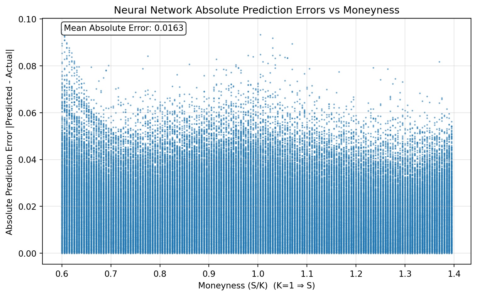
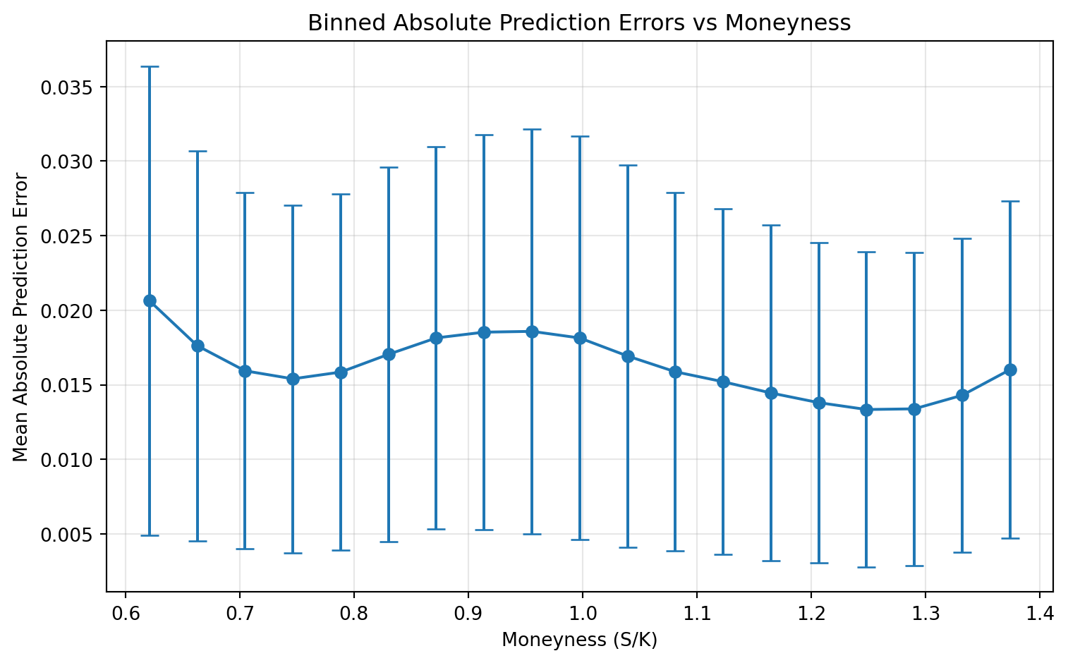
Finally, we summarize the same pattern with binned means and standard deviations of absolute error.
moneyness_bins = np.linspace(moneyness.min(), moneyness.max(), 20)
bin_centers = 0.5 * (moneyness_bins[:-1] + moneyness_bins[1:])
bin_means, _, _ = binned_statistic(moneyness, abs_err, statistic="mean", bins=moneyness_bins)
bin_stds, _, _ = binned_statistic(moneyness, abs_err, statistic="std", bins=moneyness_bins)plt.figure(figsize=(8, 5))
plt.errorbar(
bin_centers,
bin_means,
yerr=bin_stds,
fmt="o-",
capsize=5,
capthick=1,
)
plt.xlabel("Moneyness (S/K)")
plt.ylabel("Mean Absolute Prediction Error")
plt.title("Binned Absolute Prediction Errors vs Moneyness")
plt.grid(True, alpha=0.3)
plt.tight_layout()
plt.show()