Optimization in Python

Minimizing Functions

In this notebook we will learn how to minimize functions using the SciPy library optimize. Inside optimize there are many functions, one of them called minimize. Note that minimizing f(x) is the same thing as maximizing -f(x), so minimization and maximization are conceptually the same thing. The only difference is that the function minimize minimizes a function, so if we want to maximize a function we need to minimize its negative.

Let’s start by importing the libraries we will need. We will use numpy to create arrays and do some math, matplotlib to create plots, scipy.optimize to minimize functions, and yfinance to download financial data. I also add a line to ignore some warnings that we will get when downloading data from Yahoo Finance. You can ignore this line if you want, but it will make the output of the notebook cleaner.

import numpy as np
import matplotlib.pyplot as plt
from scipy.optimize import minimize
import yfinance as yf

import warnings
warnings.simplefilter(action='ignore', category=FutureWarning)

In the following we will minimize the function f(x) = x^2 - 10 x + 6. This is a second order polynomial whose second derivative is positive and therefore has a unique minimum.

In Python we can define this function as follows.

def f(x):
  return x**2 - 10*x + 6

We can plot the function by sampling f(x) at different points. Below I create a numpy array size 100 that goes from -2 to 12. I then plot f(x).

x = np.linspace(-2, 12, 100)
ax = plt.plot(x, f(x))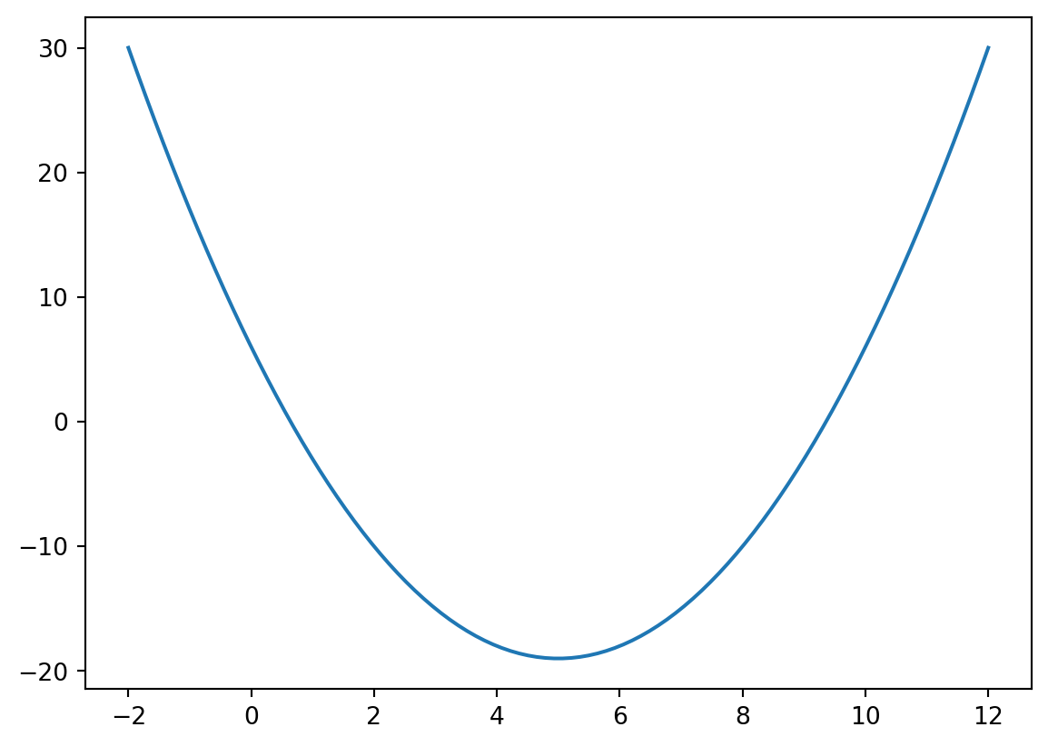

We can see that the function indeed has a unique minimum value at 5. Let’s use the routine minimize to find the minimum. The two required inputs for this routine are the function we want to minimize and an initial guess for the variables of the function.

This is a very simple function so regardless where we start we will obtain the minimum very quickly. For example, we could start from -100.

minimize(f, [-100])

  message: Optimization terminated successfully.
  success: True
   status: 0
      fun: -19.0
        x: [ 5.000e+00]
      nit: 4
      jac: [ 0.000e+00]
 hess_inv: [[ 5.000e-01]]
     nfev: 14
     njev: 7

Or we could start from 100.

minimize(f, [100])

  message: Optimization terminated successfully.
  success: True
   status: 0
      fun: -18.999999999999993
        x: [ 5.000e+00]
      nit: 4
      jac: [ 0.000e+00]
 hess_inv: [[ 5.000e-01]]
     nfev: 14
     njev: 7

In both cases we obtain the same answer. The result of the minimization is an object that we could store in a variable res.

res = minimize(f, [100])

The variable res contains the results of the optimization. We can then retrieve the solution of the optimization stored in res.x, the optimal value function given by res.fun, or to know whether the optimization was successful stored in res.success.

For example, the optimal value of the function is

res.x

array([5.00000007])

As an application of minimization, let’s compute the zeros of the previous function. An easy way to do that is to minimize the square of f(x). If the function has at least one zero, then the minimum value of the function will be zero as well. In our case we know there are two zeros. Depending on the starting value, we will find one or the other.

To start, let’s define g(x) = f(x)^2, and create a plot.

In Python we can define the function g(x) as follows.

def g(x):
  return f(x)**2

ax = plt.plot(x, g(x))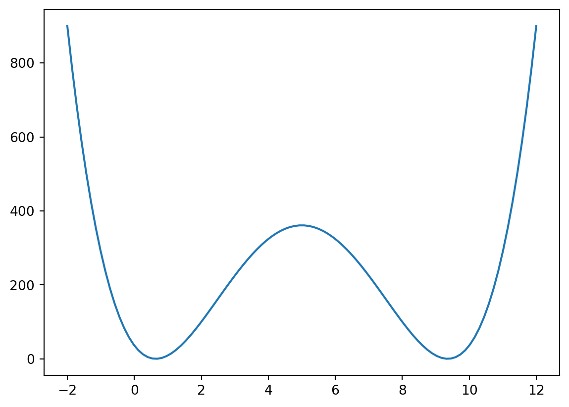

We can see that the function has two minima at which the function value is indeed zero. To find the left minimum we can start looking at -2.

minimize(g, [-2])

  message: Optimization terminated successfully.
  success: True
   status: 0
      fun: 4.0443683223940154e-13
        x: [ 6.411e-01]
      nit: 7
      jac: [-9.956e-06]
 hess_inv: [[ 6.571e-03]]
     nfev: 16
     njev: 8

With this starting point, the minimum is at x = 0.64. To find the other minimum, let’s start at 12.

minimize(g, [12])

  message: Optimization terminated successfully.
  success: True
   status: 0
      fun: 2.5606609315712264e-13
        x: [ 9.359e+00]
      nit: 7
      jac: [ 9.955e-06]
 hess_inv: [[ 6.571e-03]]
     nfev: 16
     njev: 8

The other minimum is at x = 9.36. Therefore, the two zeros of our original function are 0.64 and 9.36, which makes sense since they are symmetrical from the minimum of f(x) which is 5.

Running A Regression

A regression is a simple application of minimizing the sum of squared errors. Say a variable y depends linearly on another variable x and a random error e independent of x. The model for y is y = \alpha + \beta x + e. If we have N observations of y and x, we can estimate \alpha and \beta by minimizing \text{mse} = \sum_{i = 1}^{N} (y_i - \alpha - \beta x_i)^2.

To implement this with real data, we could try to estimate a classical factor model regression r_A = \alpha + \beta r_M + e, where M is a market index like the S&P 500 and A is a stock. In the regression, r_A and r_M represent the monthly returns of the stock and the index. I’ll use the ETF on the S&P 500 (SPY) as a proxy for M.

We first download and compute stock return data from Yahoo Finance for MSFT (stock) and SPY (proxy for S&P 500) starting from January 2000. We then compute monthly returns by resampling the data to monthly frequency and computing percentage changes. Finally, we drop the first observation as it will be NaN due to the percentage change.

df = (yf
      .download(['MSFT', 'SPY'], progress=False, start='2000-01-01')
      .loc[:,'Close']
      .resample('ME')
      .last()
      .pct_change()
      .dropna())

We can now define our objective function as the sum of squared errors.

def mse(x, dep, ind):
  return sum((dep - x[0] - x[1]*ind)**2)

Finally, the estimated alpha and beta come from minimizing this function.

minimize(mse, [0, 0], args=(df.MSFT, df.SPY))

  message: Optimization terminated successfully.
  success: True
   status: 0
      fun: 1.2319066744785045
        x: [ 3.117e-03  1.112e+00]
      nit: 3
      jac: [ 0.000e+00 -1.490e-08]
 hess_inv: [[ 1.646e-03 -6.408e-03]
            [-6.408e-03  8.458e-01]]
     nfev: 18
     njev: 6

In class I asked you to also estimate an extended version of the model. The first version we could try to estimate is: r_A = \alpha + \beta_1 r_M + \beta_2 r_M^2 + \beta_3 r_M^3 + \beta_4 r_M^4 + \beta_5 r_M^5 + e. In other words, does the error get smaller if we add powers of the independent variable?

To answer this question, let’s define a new error function that includes the powers of the independent variable.

def mse1(x, dep, ind):
  return sum((dep - x[0] - x[1]*ind - x[2]*ind**2 - x[3]*ind**3 - x[4]*ind**4 - x[5]*ind**5)**2)

We can now minimize this function. Note that the initial guess has six values as we are finding six parameters.

minimize(mse1, [0, 0, 0, 0, 0, 0], args=(df.MSFT, df.SPY))

  message: Optimization terminated successfully.
  success: True
   status: 0
      fun: 1.2171423800503955
        x: [-7.374e-04  1.310e+00  2.163e+00 -3.148e+01 -1.348e+02
             3.096e+01]
      nit: 54
      jac: [-2.682e-07  1.580e-06 -7.942e-06 -8.941e-08 -1.594e-06
            -5.201e-06]
 hess_inv: [[ 2.892e-03 -2.072e-02 ...  4.031e+01 -9.313e+00]
            [-2.072e-02  2.285e+00 ... -9.165e+02  2.103e+02]
            ...
            [ 4.031e+01 -9.165e+02 ...  2.888e+06 -6.671e+05]
            [-9.313e+00  2.103e+02 ... -6.671e+05  1.541e+05]]
     nfev: 413
     njev: 59

Clearly, the error did not go much down. It seems this new model is not that much better. We could try something else. Why not add another index and second order powers? Say we want to estimate r_A = \alpha + \beta_1 r_M + \beta_2 r_Q + \beta_3 r_M r_Q + \beta_4 r_M^2 + \beta_5 r_Q^2 + e, where Q represents the ETF on Nasdaq (QQQ). We first add Nasdaq (QQQ) to our dataframe.

df = (yf
      .download(['MSFT', 'SPY', 'QQQ'], progress=False, start='2000-01-01')
      .loc[:,'Close']
      .resample('ME')
      .last()
      .pct_change()
      .dropna())

We then modify the objective function accordingly.

def mse2(x, dep, ind1, ind2):
  return sum((dep - x[0] - x[1]*ind1 - x[2]*ind2 - x[3]*ind1*ind2 - x[4]*ind1**2 - x[5]*ind2**2)**2)

Finally we minimize the function to estimate the parameters.

minimize(mse2, [0, 0, 0, 0, 0, 0], args=(df.MSFT, df.SPY, df.QQQ))

  message: Optimization terminated successfully.
  success: True
   status: 0
      fun: 1.0457235976845725
        x: [ 1.751e-03  1.671e-01  7.294e-01  8.236e+00 -6.457e+00
            -1.352e+00]
      nit: 36
      jac: [-2.980e-08  2.757e-06 -1.580e-06 -2.384e-07 -5.811e-07
            -1.535e-06]
 hess_inv: [[ 2.416e-03 -1.252e-02 ... -4.170e-01 -1.101e-01]
            [-1.252e-02  3.022e+00 ...  1.903e+01  4.661e+00]
            ...
            [-4.170e-01  1.903e+01 ...  1.221e+03  2.538e+02]
            [-1.101e-01  4.661e+00 ...  2.538e+02  1.319e+02]]
     nfev: 273
     njev: 39

We can see that this model reduces the MSE significantly. Whether or not that is important depends on how the estimated model behaves out of sample.

Some Final Notes

The minimize function has many options that we have not explored. For example, we can set the optimization method, tolerance, and maximum number of iterations. We can also add constraints such as bounds on variables or linear restrictions. I encourage you to explore the scipy.optimize.minimize documentation for more examples.

Also, this is not the most efficient way to run a regression. In practice, we would use statsmodels, which is faster and provides richer inference output. The purpose here is to show optimization as a general finance tool: minimizing the sum of squared errors is flexible, stable in many settings, and easy to extend with regularization terms.