Class 6
A Synthetic Risk-Free Rate
A portfolio with zero variance earns the same return in every state. If markets offer no arbitrage opportunities, that return must equal the risk-free rate, r_{f} = w_{A} \mu_{A} + w_{B} \mu_{B}, \tag{3} with the weights from (2). If the zero-variance portfolio paid more than r_{f}, you could borrow at r_{f} and invest in it, earning a riskless profit with no money down. If it paid less, you would short it and lend at r_{f}. Traders would scale either trade up until prices adjusted, so perfectly correlated assets pin down a synthetic risk-free rate implied by their expected returns.
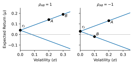
Writing R_{i} = r_{i} - r_{f} for excess returns, (3) says that w_{A} R_{A} + w_{B} R_{B} = 0 in every state, or R_{B} = \rho_{AB} \frac{\sigma_{B}}{\sigma_{A}} R_{A}. \tag{4} The excess returns of perfectly correlated assets are proportional. Taking expectations, (\mu_{B} - r_{f}) / \sigma_{B} = \rho_{AB} (\mu_{A} - r_{f}) / \sigma_{A}. With \rho_{AB} = 1 the two assets have the same Sharpe ratio and lie on the same line through r_{f}. With \rho_{AB} = -1 their Sharpe ratios are equal in size and opposite in sign, so they lie on two lines that meet at r_{f}, one rising and one falling. Figure 1 draws both cases. In each, the zero-variance portfolio is the point where the opportunity set touches the vertical axis.
Building Perfect Correlation
Perfectly correlated pairs are not something you find among traded stocks, but they are easy to build. Combining any risky asset A with the risk-free asset gives a portfolio B with r_{B} = r_{f} + w (r_{A} - r_{f}), that is, R_{B} = w R_{A}, \tag{5} so \rho_{AB} = 1 if w > 0 and \rho_{AB} = -1 if w < 0. A levered position in A is perfectly positively correlated with A, and a short position in A with the proceeds invested at r_{f} is perfectly negatively correlated with it. The set of all such portfolios is the capital allocation line of Class 4 together with its lower branch: two rays through r_{f} with slopes equal to plus and minus the Sharpe ratio of A, exactly the shape in Figure 1.
Derivatives deliver the same property over short intervals. A call option moves with its underlying asset and a put moves against it, so over a short horizon a call is perfectly positively correlated with the underlying and a put is perfectly negatively correlated with it. Combining the option with the right amount of the underlying creates an overnight risk-free position, which by the argument above must earn r_{f}. This is the no-arbitrage argument that Black, Scholes, and Merton used in 1973 to price options.
Practice Problems
Suppose that there are many assets in the security market and that the characteristics of assets A and B are given as follows:
Asset Expected Return Standard Deviation A 5% 20% B 20% 30% The correlation between the asset returns is -1. Suppose that it is possible to invest and borrow at the risk-free rate, r_{f}. What must be the value of the risk-free rate?