Class 4
The Capital Allocation Problem
Investors who share the same information should agree on the best portfolio of risky assets, but they need not agree on how much risk to take. The capital allocation decision is how much to invest in that risky portfolio Q and how much in a risk-free asset paying r_{f}. Solving it requires two ingredients: the investment opportunity set (what is feasible) and a utility function (what the investor wants).
The Capital Allocation Line
A portfolio P that invests w in Q and 1 - w in the risk-free asset has \begin{aligned} \mu_{P} & = (1 - w) r_{f} + w \mu_{Q}, \\ \sigma_{P} & = |w| \sigma_{Q}. \end{aligned} \tag{1} For w \geq 0, eliminating w gives the capital allocation line CAL(Q): \mu = r_{f} + \mathit{SR} \times \sigma, \qquad \mathit{SR} = \frac{\mu_{Q} - r_{f}}{\sigma_{Q}}, a straight line with intercept r_{f} and slope equal to the Sharpe ratio of Q, shown in Figure 1. When Q is the market portfolio, this line is the capital market line (CML).
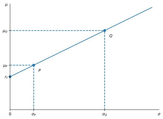
The CAL is a production function that converts risk into expected return, so the Sharpe ratio is the marginal rate of transformation of risk into expected return. Moving along the CAL by changing w does not change its slope: the Sharpe ratio depends only on the composition of the risky portfolio, not on how much of it you hold.
Mean-Variance Utility
Preferences over (\mu, \sigma) pairs are summarized by U = \mu - \frac{1}{2} A \sigma^{2}, \tag{2} where A is the coefficient of risk aversion, playing the role of relative risk aversion in the local approximation of the certainty equivalent of a small proportional gamble. Typical values are between 1 and 4.
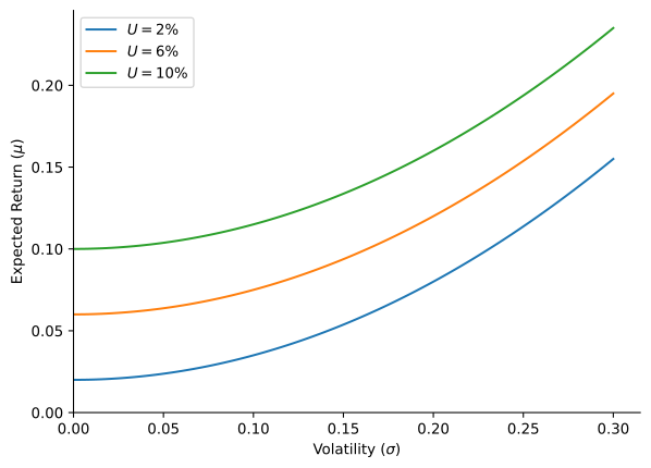
Combinations of (\mu, \sigma) giving the same utility trace an indifference curve, \mu = U + \frac{1}{2} A \sigma^{2}, an upward-sloping parabola whose intercept U is the portfolio’s certainty equivalent. Higher curves mean higher utility, as Figure 2 shows for A = 3.
Optimal Capital Allocation
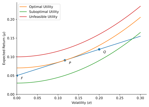
Substituting the investment opportunity set into the utility function, U = (1 - w) r_{f} + w \mu_{Q} - \frac{1}{2} A w^{2} \sigma_{Q}^{2}, the first-order condition (\mu_{Q} - r_{f}) - A w \sigma_{Q}^{2} = 0 gives w^{*} = \frac{\mu_{Q} - r_{f}}{A \sigma_{Q}^{2}}, with \mu^{*} = (1 - w^{*}) r_{f} + w^{*} \mu_{Q} and \sigma^{*} = w^{*} \sigma_{Q}. The allocation to the risky asset rises with its risk premium and falls with risk aversion and variance, which enter symmetrically. Geometrically, the optimum is the point where an indifference curve is tangent to the CAL: the marginal rate of substitution between risk and return equals the marginal rate of transformation, as illustrated in Figure 3.
Practice Problems
Investment Management Inc. (IMI) uses the capital market line to make asset allocation recommendations. IMI derives the following forecasts:
- Expected return on the market portfolio: 12%.
- Standard deviation on the market portfolio: 20%.
- Risk-free rate: 5%.
Samuel Johnson seeks IMI’s advice for a portfolio asset allocation. Johnson informs IMI that he wants the standard deviation of the portfolio to equal half of the standard deviation for the market portfolio. Using the capital market line, what expected return can IMI provide subject to Johnson’s risk constraint?
Suppose that you have $1 million and the following two opportunities from which to construct a portfolio:
- Risk-free asset earning 5% per year.
- Risky asset with expected return of 30% per year and standard deviation of 40%.
If you construct a portfolio with a standard deviation of 30%, what is its expected rate of return?
If your utility is given by U = \mu - \frac{1}{2} A \sigma^{2}, compute the optimal allocation in the risky and risk-free asset, and the expected return and standard deviation of your optimal portfolio if A = 2.