Class 7

The Tangency Portfolio

With many risky assets and no risk-free asset, the opportunity set is the hyperbola-shaped region of Class 5. Adding a risk-free asset changes it: every risky portfolio P in that region generates its own capital allocation line through r_{f} with slope equal to its Sharpe ratio. The steepest of those lines is the one that just touches the hyperbola, and we call the portfolio at that point the tangency portfolio Q. Its CAL is the efficient frontier, \mu_{P} = r_{f} + \frac{\mu_{Q} - r_{f}}{\sigma_{Q}} \sigma_{P}. \tag{1} so a portfolio is efficient only if its Sharpe ratio equals Q’s.

Beta Pricing

Take any asset P, efficient or not, and find the combination of r_{f} and Q with the same expected return. Writing \beta_{P} for the weight in Q, the difference is a residual \varepsilon_{P} with zero mean: r_{P} = (1 - \beta_{P}) r_{f} + \beta_{P} r_{Q} + \varepsilon_{P}. \tag{2} Efficiency of Q makes this residual uncorrelated with r_{Q}, which pins down the weight, \beta_{P} = \frac{\operatorname{Cov}(r_{P}, r_{Q})}{\operatorname{V}(r_{Q})}. \tag{3} Taking expectations in (2) gives the beta pricing equation \operatorname{E}(r_{P}) - r_{f} = \beta_{P} \left[ \operatorname{E}(r_{Q}) - r_{f} \right]. \tag{4} The economics is diversification, not optimization: \varepsilon_{P} adds variance without adding expected return, so it cannot earn a premium of its own. No equilibrium and no distributional assumption were used, so (4) holds for any efficient Q and every asset.

The Capital Asset Pricing Model

Beta pricing does not say which portfolio is efficient, and building Q requires estimating expected returns and inverting a large covariance matrix. The CAPM supplies the missing link. If investors all evaluate portfolios by mean and variance, share the same estimates of \pmb{\mu} and \pmb{\Sigma}, and borrow and lend at the same rate, each holds risky assets in the proportions of Q. Aggregate risky demand then has Q’s composition, and market clearing forces it to equal supply, whose composition is by definition the market portfolio M. Hence Q = M, and (4) becomes \operatorname{E}(r_{A}) - r_{f} = \beta_{A} \left[ \operatorname{E}(r_{M}) - r_{f} \right], \qquad \beta_{A} = \frac{\operatorname{Cov}(r_{A}, r_{M})}{\operatorname{V}(r_{M})} = \frac{\sigma_{A} \rho_{A,M}}{\sigma_{M}}. \tag{5} Market-value weights require no estimate of expected returns or covariances, which is the practical payoff. The line in (5) is the security market line (SML). Inefficient assets lie below the CAL in the (\sigma, \mu) diagram, but exactly on the SML in the (\beta, \mu) diagram: efficiency is a property an asset can fail, beta pricing is not.

Figure 1: Two risky assets and a risk-free asset of 4\%. Assets A and B lie below the CAL on the left, since neither is efficient, but exactly on the SML on the right.

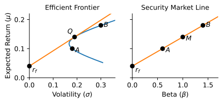
The assumptions are strong. If investors disagree about expected returns or face different borrowing rates, they need not hold the same risky portfolio, and nothing forces M to be efficient. Beta pricing survives all of this; only the identification Q = M is at risk.

Practice Problems

1. The risk-free rate is 3% and the market portfolio has an expected return of 11% with a volatility of 15%. Stock A has a volatility of 45% and a correlation of 0.4 with the market.

   1. Compute \beta_{A} and the expected return of A predicted by the CAPM.
   2. What fraction of A’s variance is systematic? What is the volatility of its firm-specific return?
   3. Is A an efficient portfolio? Explain.

2. You know that the tangency portfolio Q has an expected return of 16% and a volatility of 25%, and that the risk-free rate is 4%. A fund F has a beta of 0.8 with respect to Q and a volatility of 30%.

   1. What is the expected return of F?
   2. Build a portfolio of Q and the risk-free asset with the same expected return as F. What is its volatility? Why is it lower than 30%?