Class 3

Utility Functions

In a single-period model, preferences over consumption are represented by a smooth utility function u: \mathbb{R}^{+} \rightarrow \mathbb{R}. We will use two common families:

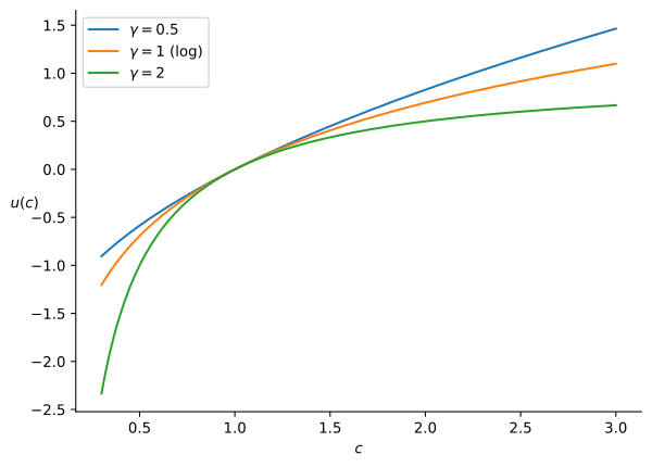
Power utility (with log utility as the limiting case): u(c) = \dfrac{c^{1 - \gamma} - 1}{1 - \gamma}, \quad \gamma > 0, \gamma \neq 1, and u(c) = \ln(c) when \gamma = 1.
Exponential utility: u(c) = -e^{-a c}, \quad a > 0.

Both families are increasing and strictly concave, so the marginal utility of an extra unit of consumption is positive but decreasing. The parameters \gamma and a control how concave the function is, and as we will see, how averse the agent is to risk. Figure 1 plots the power family for three values of \gamma.

Three increasing, concave curves plotting power utility u of c against consumption c, for gamma equal to 0.5, 1 (log utility), and 2. All three pass through the point where c equals 1. Higher values of gamma produce a more curved, more concave function. — Figure 1: Power utility for different values of \gamma.

Expected Utility and Risk Aversion

Denote by \overset{\sim}{W} the agent’s random end-of-period wealth. Since utility is random too, we rank outcomes by expected utility, U(\overset{\sim}{W}) = \operatorname{E}(u(\overset{\sim}{W})).

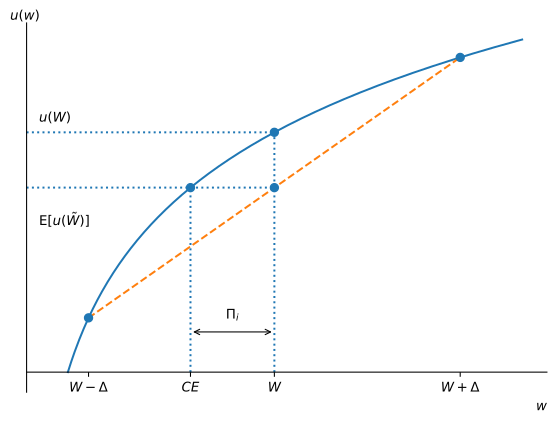
For a risk \tilde{\varepsilon} with \operatorname{E}(\tilde{\varepsilon}) = 0 and \operatorname{V}(\tilde{\varepsilon}) > 0, the agent is risk averse if she prefers certain wealth W to the gamble W + \tilde{\varepsilon}: u(W) > \operatorname{E}(u(W + \tilde{\varepsilon})). \tag{1} By Jensen’s inequality, (1) holds for every such gamble if and only if u is strictly concave. Figure 2 illustrates: expected utility is the chord’s height at W, which concavity places strictly below the curve.

A concave logarithmic utility curve with a dashed chord joining the utility at W minus Delta and W plus Delta. The midpoint of the chord at W is the expected utility of the gamble and lies strictly below the curve at u of W. Reading that expected utility back across to the curve gives the certainty equivalent CE, which is well to the left of W. The horizontal gap between CE and W is labeled as the insurance premium. — Figure 2: A concave utility function, Jensen’s inequality, and the insurance premium.

The Insurance Premium

An agent facing the risk \tilde{\varepsilon} on wealth W is indifferent between bearing it and paying \Pi_{i} to insure it when u(W - \Pi_{i}) = \operatorname{E}(u(W + \tilde{\varepsilon})). \tag{2} \Pi_{i} is the insurance premium, and W - \Pi_{i} is the gamble’s certainty equivalent.

Comparing premiums only ranks risk aversion across agents facing the same gamble at the same wealth; for one agent, \Pi_i varies with W, so premiums at different wealth levels say nothing about a change in her risk aversion.

Local Risk Aversion

For a small, fair gamble \tilde{\varepsilon} with \operatorname{E}(\tilde{\varepsilon}) = 0, \operatorname{V}(\tilde{\varepsilon}) = \sigma_{\varepsilon}^{2} on wealth W, a Taylor expansion of (2) gives \Pi_{i} \approx \frac{1}{2} \mathit{ARA} \cdot \sigma_{\varepsilon}^{2}, \qquad \mathit{ARA} = -\frac{u''(W)}{u'(W)}. \mathit{ARA} is the coefficient of absolute risk aversion: the dollar premium the agent pays per unit of variance. An agent with decreasing absolute risk aversion pays a smaller dollar premium as her wealth grows.

For a proportional gamble \tilde{\varepsilon} = W \tilde{\delta} (a percentage shock with \operatorname{V}(\tilde{\delta}) = \sigma_{\delta}^{2}), the premium as a share of wealth is \frac{\Pi_{i}}{W} \approx \frac{1}{2} \mathit{RRA} \cdot \sigma_{\delta}^{2}, \qquad \mathit{RRA} = -\frac{u''(W)}{u'(W)} W, the coefficient of relative risk aversion. An agent with constant relative risk aversion (CRRA) keeps a fixed fraction of wealth in risky assets regardless of her wealth level.

Practice Problems

Suppose your utility function is logarithmic, u(W) = \ln W, and your current wealth is $4,000.
1. You face a 50/50 chance of either gaining or losing $1,000. You have the option to purchase an insurance policy that completely eliminates this risk. What is the maximum amount you would be willing to pay for this insurance policy?
2. Assume you did not buy the insurance and ended up losing, reducing your wealth to $3,000. If you are presented with the same gamble again, what is the maximum amount you would be willing to pay for insurance this time?
3. Explain the difference between the amounts found in parts (a) and (b).
An entrepreneur faces a 1% chance that a fire will reduce her net worth to $1, and a 99% chance that her net worth will remain at $100,000. Her utility function is logarithmic, u(W) = \ln W. She is evaluating an insurance policy that would pay $99,999 in the event of a fire and nothing otherwise. Determine the maximum amount she would be willing to pay for this insurance policy.