Class 5
Portfolios of Two Risky Assets
In Class 4 the risky portfolio Q was taken as given. We now ask where it comes from, starting with two risky assets A and B. A portfolio P that invests 1 - w in A and w in B earns r_{P} = (1 - w) r_{A} + w r_{B}, so that \begin{aligned} \mu_{P} & = (1 - w) \mu_{A} + w \mu_{B}, \\ \sigma_{P}^{2} & = (1 - w)^{2} \sigma_{A}^{2} + w^{2} \sigma_{B}^{2} + 2 w (1 - w) \sigma_{AB}, \end{aligned} \tag{1} where \sigma_{AB} = \sigma_{A} \sigma_{B} \rho_{AB} is the covariance of returns. We assume throughout that short-selling is allowed, so w can be negative (short B to overinvest in A) or greater than one (short A to overinvest in B).
The expected return is a linear combination of \mu_{A} and \mu_{B}, but volatility is not. The cross term 2 w (1 - w) \sigma_{AB} can add to or subtract from portfolio risk depending on the weights as much as on the correlation: holding both assets long lowers risk when \rho_{AB} < 0, while holding one of them short lowers risk when \rho_{AB} > 0. Diversification is choosing the weights that exploit whatever correlation the assets have.
The Investment Opportunity Set
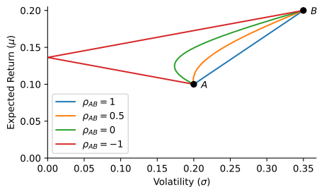
Letting w range over the real line traces out the investment opportunity set of A and B, a hyperbola in (\sigma, \mu) space, drawn in Figure 1 for long positions in both assets. The lower the correlation, the further the curve bows to the left of the segment AB. When |\rho_{AB}| = 1 the hyperbola degenerates into straight lines and the right weights make the portfolio riskless: long-only if \rho_{AB} = -1, long-short if \rho_{AB} = 1.
In practice, stock returns are almost always positively correlated with one another, so a negative correlation is rarely something you find. It is something you build: an inverse ETF, or any short position, delivers it by construction, which is the same trade as holding one asset short in the formulas above.
The Minimum-Variance Portfolio
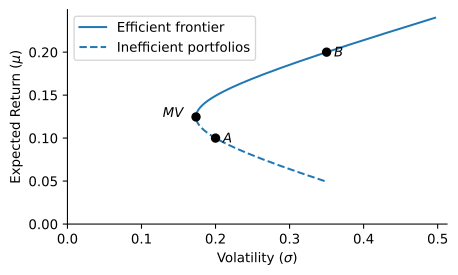
Every opportunity set has a leftmost point, the minimum-variance portfolio (MVP). Minimizing (1) with respect to w gives the first-order condition -(1 - w) \sigma_{A}^{2} + w \sigma_{B}^{2} + (1 - 2 w) \sigma_{AB} = 0, and therefore w_{A} = \frac{\sigma_{B}^{2} - \sigma_{AB}}{\sigma_{A}^{2} + \sigma_{B}^{2} - 2 \sigma_{AB}}, \qquad w_{B} = \frac{\sigma_{A}^{2} - \sigma_{AB}}{\sigma_{A}^{2} + \sigma_{B}^{2} - 2 \sigma_{AB}}. \tag{2} When |\rho_{AB}| = 1 the denominator collapses to (\sigma_{A} \mp \sigma_{B})^{2} and (2) returns the zero-variance portfolio of the previous section. The weights depend only on the covariance matrix, not on expected returns, and each is decreasing in its own asset’s variance and in the covariance with the other asset.
Portfolios on the frontier above the MVP are efficient: no other portfolio in the set offers more expected return at the same volatility. Portfolios below the MVP are dominated, since moving up along the curve raises \mu while lowering \sigma. Figure 2 illustrates both regions.
Many Risky Assets
With N assets, collect the weights in a vector \pmb{w} satisfying \pmb{w}^{\top} \mathbf{1} = 1, the expected returns in \pmb{\mu}, and the covariances in the N \times N matrix \pmb{\Sigma} whose (i, j) entry is \operatorname{Cov}(r_{i}, r_{j}). Then \mu_{P} = \pmb{w}^{\top} \pmb{\mu}, \qquad \sigma_{P}^{2} = \pmb{w}^{\top} \pmb{\Sigma} \pmb{w}, \qquad \operatorname{Cov}(r_{P}, r_{Q}) = \pmb{w}_{P}^{\top} \pmb{\Sigma} \pmb{w}_{Q}, \tag{3} which reduce to (1) when N = 2. The budget constraint leaves N - 1 degrees of freedom, so the opportunity set is now a filled region whose left boundary is again a hyperbola, the minimum-variance frontier. Adding the risk-free asset of Class 4 will single out one portfolio on its efficient upper branch: the one with the highest Sharpe ratio.
How Far Can Diversification Go?
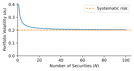
Take the special case of N securities held in equal proportions, w_{i} = 1/N. Separating the N diagonal terms of the quadratic form in (3) from the N (N - 1) off-diagonal ones, \sigma_{P}^{2} = \frac{1}{N} (\text{Average Variance}) + \frac{N - 1}{N} (\text{Average Covariance}), \tag{4} so that as N grows the first term vanishes and \sigma_{P}^{2} \xrightarrow[N \to \infty]{} \text{Average Covariance}. Individual variance is diversifiable (or firm-specific) risk, while the average covariance is systematic risk that no amount of diversification removes. As Figure 3 shows, most of the gain is exhausted well before 30 securities, and only uncorrelated securities would drive portfolio risk to zero.
Practice Problems
Consider two risky assets A and B for which you have the following information.
Asset Expected Return Standard Deviation A 15% 30% B 25% 40% The correlation between the assets returns is 0.3.
- If you invest 40% in A and 60% in B, compute the expected return and standard deviation of your portfolio.
- Compute the weights, expected return and standard deviation of the minimum variance portfolio.
A portfolio manager follows a large universe of stocks. Each stock has a variance of returns of 0.25, and the average covariance between the returns of any two stocks in the universe is 0.10. The manager forms equally-weighted portfolios out of this universe.
Compute the volatility of an equally-weighted portfolio of N = 20 stocks.
What volatility does the portfolio approach as N becomes arbitrarily large? What fraction of the variance of a single stock has been diversified away in the limit?
Suppose instead that the stocks were uncorrelated with each other. What would the answer to part (b) be in that case?