Pricing with Jumps
The geometric Brownian motion of the previous notes has continuous paths, so a stock price can never move by a large amount in a short time. Real prices do. Stocks gap on earnings announcements, markets crash, and firms default, and options markets price these risks: out-of-the-money puts trade at much higher implied volatilities than the Black-Scholes model can explain. Adding the jumps of the Poisson process to the Brownian motion of the stock price produces a jump-diffusion, the model of Merton (1976).
These notes bring together the two halves of the course. The Poisson process supplies the jumps, its exponential martingale supplies the change of measure, and its characteristic function supplies the pricing method. We first describe the Merton model and the distribution of its returns, extend Itô’s formula to processes with jumps, and show how to change the intensity of a Poisson process. We then apply these tools to credit spreads and to options, where jumps make the market incomplete. The last section prices options by inverting the characteristic function of the log price, the method used in practice for models with jumps. These notes draw on Shreve (2004) and Duffie and Singleton (1999).
The Merton Model
Stock Prices with Jumps
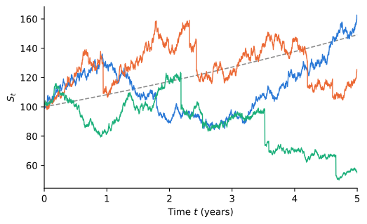
Let \{N_{t}\} be a Poisson process with intensity \lambda, and let Y_{1}, Y_{2}, \ldots be iid \mathcal{N}(m, s^{2}) random variables, independent of N and of the Brownian motion B. In the model of Merton (1976), the stock price is S_{t} = S_{0} \exp\left(\left(\mu - \tfrac{1}{2} \sigma^{2} - \lambda k\right) t + \sigma B_{t} + \sum_{i = 1}^{N_{t}} Y_{i}\right), \qquad k = \operatorname{E}(e^{Y}) - 1 = e^{m + \frac{1}{2} s^{2}} - 1. \tag{1} Between jumps, the price is a geometric Brownian motion with volatility \sigma. At the time of the i-th event of the Poisson process, the log price jumps by Y_{i}, so the price is multiplied by e^{Y_{i}}, a percentage change of e^{Y_{i}} - 1. The constant k is the expected percentage jump, and with m < 0 jumps are mostly down, as in a crash.
The term -\lambda k in the drift ensures that \mu is still the expected return. Since B, N, and the Y_{i} are independent, \operatorname{E}(S_{t}) = S_{0} e^{(\mu - \lambda k) t} \, \operatorname{E}\left(e^{\sigma B_{t} - \frac{1}{2} \sigma^{2} t}\right) \operatorname{E}\left(e^{\sum_{i = 1}^{N_{t}} Y_{i}}\right) = S_{0} e^{(\mu - \lambda k) t} \times 1 \times e^{\lambda t (M_{Y}(1) - 1)} = S_{0} e^{\mu t}, where the last expectation is the MGF of a compound Poisson process from the notes on Poisson processes, evaluated at \theta = 1, and M_{Y}(1) = 1 + k. Jumps add to the expected return at the rate \lambda k, so without the correction, the stock would earn \mu + \lambda k. Applying the same argument conditionally on \mathcal{F}_{t}, the process S_{t} e^{-\mu t} is a martingale.
The Distribution of Returns
The log return X_{t} = \ln(S_{t} / S_{0}) is the sum of a normal random variable and an independent compound Poisson process. Its characteristic function is the product of the two, using the example on the Merton model in the notes on Poisson processes: \phi_{X_{t}}(u) = \exp\left(i u \left(\mu - \tfrac{1}{2} \sigma^{2} - \lambda k\right) t - \tfrac{1}{2} u^{2} \sigma^{2} t + \lambda t \left(e^{i u m - \frac{1}{2} u^{2} s^{2}} - 1\right)\right). \tag{2} Conditional on N_{t} = n, the log return is normal with mean \left(\mu - \frac{1}{2} \sigma^{2} - \lambda k\right) t + n m and variance \sigma^{2} t + n s^{2}. Its density is therefore a mixture of normal densities, weighted by the Poisson probabilities of n jumps.
The cumulant generating function K(\theta) = \ln \operatorname{E}(e^{\theta X_{t}}) is the logarithm of the same expression with i u replaced by \theta. The normal part contributes only to the first two cumulants, so every cumulant beyond the variance comes from the jumps. Writing \kappa_{j} for the j-th cumulant, the Poisson part contributes \lambda t \operatorname{E}(Y^{j}) to each, so \kappa_{2} = \sigma^{2} t + \lambda t (m^{2} + s^{2}), \qquad \kappa_{3} = \lambda t \left(m^{3} + 3 m s^{2}\right), \qquad \kappa_{4} = \lambda t \left(m^{4} + 6 m^{2} s^{2} + 3 s^{4}\right). The skewness \kappa_{3} / \kappa_{2}^{3/2} is negative when m < 0, and the excess kurtosis \kappa_{4} / \kappa_{2}^{2} is positive, so the tails are heavier than normal. Both shrink as the horizon grows, like 1 / \sqrt{t} and 1 / t. Over long horizons many jumps average out and returns look normal, but over short horizons a single jump dominates. This is why jumps matter most for short-dated options.
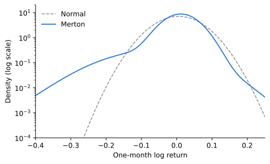
With the parameters of Figure 1, the one-month log return has skewness -1.31 and excess kurtosis 5.75. A normal distribution with the same variance underestimates the probability of large losses by orders of magnitude, as Figure 2 shows.
Itô’s Formula with Jumps
Processes with Jumps
Consider a process that follows an Itô process between jumps and jumps by Z_{i} at the i-th event of a Poisson process: X_{t} = X_{0} + \int_{0}^{t} a_{s} \mathop{}\!\mathrm{d}s + \int_{0}^{t} b_{s} \mathop{}\!\mathrm{d}B_{s} + \sum_{i = 1}^{N_{t}} Z_{i}. Write X_{t-} for the value just before time t and \Delta X_{t} = X_{t} - X_{t-} for the jump at time t, which is zero except at the event times. The log price in (1) has this form, with constant coefficients and Z_{i} = Y_{i}.
Over a short interval \mathop{}\!\mathrm{d}t, an event occurs with probability \lambda \mathop{}\!\mathrm{d}t+ o(\mathop{}\!\mathrm{d}t), so the expected change from the jumps is \lambda \operatorname{E}(Z) \mathop{}\!\mathrm{d}t. This gives the rule that replaces “the drift is zero” for processes with jumps.
The proof is the same as for the compensated Poisson process N_{t} - \lambda t. The compound Poisson process has independent increments, and its expected increase over (s, t] is \lambda (t - s) \operatorname{E}(Z) by the moments of a compound Poisson process. The martingale N_{t} - \lambda t is the case Z_{i} = 1. As in the notes on Poisson processes, the expected jump \lambda \operatorname{E}(Z) \mathop{}\!\mathrm{d}t is called the compensator of the jumps.
The Formula
Between events, X is an ordinary Itô process, and Itô’s formula from the notes on stochastic calculus applies. At an event time, X jumps from X_{t-} to X_{t-} + \Delta X_{t}, and a function of X jumps from f(X_{t-}) to f(X_{t-} + \Delta X_{t}). There are finitely many events in any interval, so adding the two kinds of changes gives the formula.
The jump term uses the exact change in f, not a Taylor expansion, because a jump is not small. The quadratic variation of the jumps is \sum (\Delta X_{s})^{2}, which was the result [N, N]_{t} = N_{t} in the notes on Poisson processes, and the full change f(X_{s-} + \Delta X_{s}) - f(X_{s-}) accounts for this and all higher powers at once.
Example 1 Apply the formula to S_{t} = e^{X_{t}}, where X_{t} is the log price in (1), with a = \mu - \frac{1}{2} \sigma^{2} - \lambda k, b = \sigma, and jumps Y_{i}. Between jumps, Itô’s formula gives \mathop{}\!\mathrm{d}S_{t} = S_{t} \left((\mu - \lambda k) \mathop{}\!\mathrm{d}t+ \sigma \mathop{}\!\mathrm{d}B_{t}\right), as for a GBM. At a jump, S changes by e^{X_{t-} + Y_{i}} - e^{X_{t-}} = S_{t-} (e^{Y_{i}} - 1). In differential notation, \frac{\mathop{}\!\mathrm{d}S_{t}}{S_{t-}} = (\mu - \lambda k) \mathop{}\!\mathrm{d}t+ \sigma \mathop{}\!\mathrm{d}B_{t} + \left(e^{Y} - 1\right) \mathop{}\!\mathrm{d}N_{t}, where \mathop{}\!\mathrm{d}N_{t} equals one at an event and zero otherwise. The expected percentage jump is k and jumps arrive at rate \lambda, so the compensator of the jump term is \lambda k \mathop{}\!\mathrm{d}t. The total expected return is \mu - \lambda k + \lambda k = \mu, as computed directly above.
The same reasoning extends the product rule. At a common jump time of two processes, their product changes by \Delta (X Y) = X_{t-} \Delta Y + Y_{t-} \Delta X + \Delta X \, \Delta Y, which is the exact change of x y and has the same form as the continuous product rule.
Changing the Jump Intensity
Girsanov’s theorem for Brownian motion reweights paths with the exponential martingale e^{-\theta B_{t} - \frac{1}{2} \theta^{2} t} and shifts the drift. The Poisson process has its own exponential martingale, e^{\theta N_{t} - \lambda t (e^{\theta} - 1)}, and reweighting paths with it changes the intensity.
Proof
With e^{\theta} = \lambda^{*} / \lambda, we have \lambda (e^{\theta} - 1) = \lambda^{*} - \lambda, so Z_{t} is the exponential martingale of the Poisson process. As in the proof of Girsanov’s theorem, \operatorname{E}^{*}(W) = \operatorname{E}(Z_{t} W) for any W known at time t. For s < t and real u and v, write \Delta N = N_{t} - N_{s} and split Z_{t} into a factor depending on N_{s} and a factor depending on \Delta N, which are independent. For the first factor, \operatorname{E}\left(\left(\tfrac{\lambda^{*}}{\lambda}\right)^{N_{s}} e^{-(\lambda^{*} - \lambda) s} e^{u N_{s}}\right) = e^{-(\lambda^{*} - \lambda) s} \, e^{\lambda s \left(\frac{\lambda^{*}}{\lambda} e^{u} - 1\right)} = e^{\lambda^{*} s (e^{u} - 1)}, using the MGF of a Poisson random variable. The second factor equals e^{\lambda^{*} (t - s) (e^{v} - 1)} in the same way. Therefore, the joint MGF of N_{s} and \Delta N under \operatorname{P}^{*} factors into the MGFs of independent Poisson random variables with means \lambda^{*} s and \lambda^{*} (t - s), which is the definition of a Poisson process with intensity \lambda^{*}. The same calculation applies to any finite number of increments.A Brownian change of measure can only shift the drift, because the quadratic variation of Brownian motion is the same on every path. The quadratic variation of the Poisson process, [N, N]_{t} = N_{t}, is random, so reweighting paths can change how often jumps occur. Paths with many events receive more weight when \lambda^{*} > \lambda, so jumps become more frequent. Since Z_{T} > 0, the two measures agree on which events are impossible.
The same idea can also change the distribution of the jump sizes. If the sizes have density g under \operatorname{P} and we want density g^{*} under \operatorname{P}^{*}, we multiply Z_{t} by \prod_{i \leq N_{t}} g^{*}(Y_{i}) / g(Y_{i}). Brownian motion and jumps can be reweighted at the same time, since independent sources of randomness can be reweighted separately. In general, a change of measure in a jump-diffusion can shift the Brownian drift, change the intensity, and change the distribution of jump sizes.
Application: Credit Spreads
The notes on Poisson processes priced a defaultable zero-coupon bond by discounting its expected payoff at the risk-free rate, obtaining a credit spread equal to the default intensity. We can now include a premium for default risk.
A firm defaults at the first event \tau of a Poisson process with intensity \lambda under \operatorname{P}. Defaults tend to happen in bad times, when a dollar is more valuable, so we let the SDF jump up at default. Specifically, let \Lambda_{t} = e^{-r t} (1 + \eta)^{N_{t}} e^{-\lambda \eta t}, \qquad \eta > -1, which jumps by the factor 1 + \eta at each event. The second and third factors form the exponential martingale of the Poisson process with e^{\theta} = 1 + \eta, so \Lambda_{t} e^{r t} is a martingale and the SDF has drift -r, as required. When \eta > 0, a dollar received just after default is worth more than a dollar received just before.
The bond pays one dollar at T if the firm survives. At default, the bond loses a fraction L of its value, so bondholders recover the fraction 1 - L, and we suppose the recovered amount is then invested at the risk-free rate. Guess that before default the bond price is P_{t} = e^{-c (T - t)} for some yield c. The pricing equation of the notes on discount factors requires \Lambda P to have zero expected change. Before default, \Lambda P has continuous drift \Lambda P \left(-r - \lambda \eta + c\right) \mathop{}\!\mathrm{d}t. At default, \Lambda is multiplied by 1 + \eta and P by 1 - L, so \Lambda P changes by \Lambda P \left((1 + \eta)(1 - L) - 1\right), with intensity \lambda. Setting the total expected change to zero, -r - \lambda \eta + c + \lambda \left((1 + \eta)(1 - L) - 1\right) = 0 \quad \Longleftrightarrow \quad c = r + \lambda (1 + \eta) L. Writing \lambda^{*} = \lambda (1 + \eta), the credit spread is c - r = \lambda^{*} L. \tag{3}
The same result follows from a change of measure. The risk-neutral density is \Lambda_{t} \beta_{t} = (1 + \eta)^{N_{t}} e^{-\lambda \eta t}, which is the density Z_{t} of the previous section with \lambda^{*} / \lambda = 1 + \eta. Under the risk-neutral measure, default arrives with intensity \lambda^{*} = \lambda (1 + \eta), and the bond is priced by discounting at the risk-free rate. With zero recovery, L = 1, this gives P = e^{-(r + \lambda^{*}) T}, the formula of the notes on Poisson processes with the risk-neutral intensity \lambda^{*} in place of the historical intensity \lambda.
The spread (3) exceeds the expected loss rate \lambda L by the factor 1 + \eta, the compensation investors require for bearing default risk that is concentrated in bad times. Spreads on investment-grade corporate bonds are typically several times the expected loss rate, which points to large values of \eta.
Option Pricing in the Merton Model
Jumps Make the Market Incomplete
In the Black-Scholes model, an option can be replicated by trading the stock, because the option and the stock respond to the same single source of risk. With jumps this fails. A position in the stock can offset the exposure of an option to \mathop{}\!\mathrm{d}B, but not its exposure to a jump of random size: the change in an option’s value at a jump is a nonlinear function of the jump size, while the change in the stock position is linear in e^{Y} - 1. The market is incomplete, and no-arbitrage alone does not determine option prices.
In terms of the previous section, many SDFs price the stock correctly. Each one implies a risk-neutral measure under which the discounted stock price is a martingale, which by the compensated jump rule means \frac{\mathop{}\!\mathrm{d}S_{t}}{S_{t-}} = (r - \lambda^{*} k^{*}) \mathop{}\!\mathrm{d}t+ \sigma \mathop{}\!\mathrm{d}B_{t}^{*} + \left(e^{Y} - 1\right) \mathop{}\!\mathrm{d}N_{t}, where under \operatorname{P}^{*} the jumps arrive at intensity \lambda^{*} and have expected percentage size k^{*}. Different choices of \lambda^{*} and of the jump distribution give different option prices. Choosing among them is an economic assumption about how investors price jump risk, or, in practice, a matter of calibrating the risk-neutral parameters to observed option prices.
Merton (1976) assumed that jump risk is specific to the firm and can be diversified away, so investors require no premium for it. The SDF then does not jump, and only the Brownian drift changes under the risk-neutral measure. The intensity and the jump distribution are the same under \operatorname{P} and \operatorname{P}^{*}, and \frac{\mathop{}\!\mathrm{d}S_{t}}{S_{t-}} = (r - \lambda k) \mathop{}\!\mathrm{d}t+ \sigma \mathop{}\!\mathrm{d}B_{t}^{*} + \left(e^{Y} - 1\right) \mathop{}\!\mathrm{d}N_{t}. Under this measure, S_{T} has the form (1) with \mu replaced by r.
Merton’s Formula
Conditional on N_{T} = n, the log price under \operatorname{P}^{*} is normal with mean \ln S_{0} + \left(r - \lambda k - \frac{1}{2} \sigma^{2}\right) T + n m and variance \sigma^{2} T + n s^{2}. A call is therefore a Poisson mixture of options in Black-Scholes models with different volatilities and interest rates.
Proof
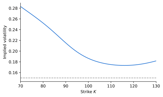
In a Black-Scholes model with rate r_{n} and volatility \sigma_{n}, the log price is normal with mean \ln S_{0} + (r_{n} - \frac{1}{2} \sigma_{n}^{2}) T and variance \sigma_{n}^{2} T. Since \ln(1 + k) = m + \frac{1}{2} s^{2}, \left(r_{n} - \tfrac{1}{2} \sigma_{n}^{2}\right) T = (r - \lambda k) T + n \left(m + \tfrac{1}{2} s^{2}\right) - \tfrac{1}{2} \sigma^{2} T - \tfrac{1}{2} n s^{2} = \left(r - \lambda k - \tfrac{1}{2} \sigma^{2}\right) T + n m, and \sigma_{n}^{2} T = \sigma^{2} T + n s^{2}. Conditional on N_{T} = n, the log price therefore has the same distribution as in that Black-Scholes model. The Black-Scholes price discounts at r_{n}, so e^{-r T} \operatorname{E}^{*}\left((S_{T} - K)^{+} \mid N_{T} = n\right) = e^{(r_{n} - r) T} \, C^{BS}(S_{0}, K, r_{n}, \sigma_{n}, T). Averaging over the Poisson distribution of N_{T}, C = \sum_{n = 0}^{\infty} e^{-\lambda T} \frac{(\lambda T)^{n}}{n!} e^{-\lambda k T} (1 + k)^{n} \, C^{BS}(S_{0}, K, r_{n}, \sigma_{n}, T), and e^{-\lambda T} e^{-\lambda k T} (\lambda T)^{n} (1 + k)^{n} = e^{-\lambda' T} (\lambda' T)^{n}.Example 3 Take the Merton model of Figure 1 with S_{0} = 100, r = 0.05, and a three-month at-the-money call, K = 100 and T = 0.25. Merton’s formula gives a price of 4.3499, compared with 3.6351 in a Black-Scholes model with the diffusion volatility \sigma = 0.15 alone. Inverting the Black-Scholes formula, the Merton price corresponds to an implied volatility of 0.1865. A three-month put with strike 80 is worth 0.1342 in the Merton model and only 0.0015 without jumps.
The implied volatility depends on the strike. Figure 3 plots it for three-month options. Low strikes, which pay off after a crash, have the highest implied volatilities, because downward jumps make large losses far more likely than the lognormal distribution allows. This pattern, called the volatility skew, has been a persistent feature of index options since the crash of 1987, and the Black-Scholes model, with a single volatility for all strikes, cannot produce it.
Fourier Pricing
Prices from Characteristic Functions
Merton’s formula works because, given the number of jumps, the log price is normal. For most models with jumps or stochastic volatility the density of the log price is not known in closed form, but its characteristic function is, as (2) illustrates. The notes on generating functions noted that probabilities can be recovered from the characteristic function by inversion. This is the basis of option pricing in such models.
The pricing notes wrote the price of a call as C = S_{0} \operatorname{P}^{S}(S_{T} > K) - K e^{-r T} \operatorname{P}^{*}(S_{T} > K), using the risk-neutral measure \operatorname{P}^{*} and the measure \operatorname{P}^{S} that uses the stock as the unit of account. The derivation did not depend on the Black-Scholes model, so the formula holds in any model with a risk-neutral measure. Both probabilities can be computed from the characteristic function of X = \ln S_{T} under \operatorname{P}^{*}.
Proof
The Dirichlet integral \int_{0}^{\infty} \frac{\sin(a u)}{u} \mathop{}\!\mathrm{d}u equals \frac{\pi}{2} if a > 0 and -\frac{\pi}{2} if a < 0. Therefore, for y \neq x, \mathbf{1}_{\{y > x\}} = \frac{1}{2} + \frac{1}{\pi} \int_{0}^{\infty} \frac{\sin(u (y - x))}{u} \mathop{}\!\mathrm{d}u. Setting y = X, taking expectations, and interchanging the expectation and the integral, which can be justified, \operatorname{P}(X > x) = \frac{1}{2} + \frac{1}{\pi} \int_{0}^{\infty} \frac{\operatorname{E}\left(\sin(u (X - x))\right)}{u} \mathop{}\!\mathrm{d}u. Finally, \operatorname{E}(\sin(u (X - x))) is the imaginary part of \operatorname{E}(e^{i u (X - x)}) = e^{-i u x} \phi(u).The formula gives \operatorname{P}^{*}(S_{T} > K) directly, with x = \ln K and \phi the risk-neutral characteristic function of \ln S_{T}. For \operatorname{P}^{S} we need the characteristic function of \ln S_{T} under the stock measure, whose density with respect to \operatorname{P}^{*} is S_{T} / \operatorname{E}^{*}(S_{T}) = e^{X} / \phi(-i), with \phi(-i) = \operatorname{E}^{*}(e^{X}) = S_{0} e^{r T}. Therefore, \phi^{S}(u) = \operatorname{E}^{*}\left(\frac{e^{X}}{\phi(-i)} e^{i u X}\right) = \frac{\phi(u - i)}{\phi(-i)}. The change of numeraire, which in the Black-Scholes model shifted the drift of the log price by \sigma^{2}, becomes a shift in the argument of the characteristic function.
Example 4 For the at-the-money call of Example 3, numerical integration of the Fourier pricing formula with the characteristic function (2), with \mu replaced by r, gives \Pi_{1} = 0.6092 and \Pi_{2} = 0.5728, and a call price of C = 100 \times 0.6092 - 100 e^{-0.05 \times 0.25} \times 0.5728 = 4.3499, which matches the value 4.3499 from Merton’s formula.
Why Fourier Methods
The Fourier formula needs nothing from the model except the characteristic function of the log price. Any model in which that function has a closed form can be priced the same way, including models with other jump distributions and the stochastic volatility model of Heston (1993). This is why the characteristic function, which in the notes on Poisson processes was a convenient way to describe a compound Poisson process, becomes the central object in modern option pricing. In practice, related formulas evaluated with the fast Fourier transform price options at many strikes at once, which makes it fast to calibrate a model’s risk-neutral parameters to an entire set of option prices.