Derivatives Pricing in Continuous Time
The previous notes showed that the stochastic discount factor has drift -r and that every risk premium equals minus the covariance of a return with the SDF. These notes turn that result into a pricing method. Girsanov’s theorem, from the notes on stochastic calculus, uses the SDF to build a new probability measure under which every asset earns the risk-free rate. Under this risk-neutral measure, the price of any asset is its expected payoff discounted at the risk-free rate, the familiar rule from the start of the notes on discount factors, now valid for risky payoffs.
We apply the method to bonds, futures, and forwards, and then to the model of Black and Scholes (1973), where it delivers the Black-Scholes formula for European options. The same model also yields the partial differential equation that every derivative price satisfies, which is how Black and Scholes originally derived their formula.
Price Processes
Let’s start considering a non-dividend paying stock S over the time interval [0, T]. Of course, a stock that does not pay dividends forever is a bubble but we will focus on a finite period of time in which the stock does not pay dividends. The stock price process follows a geometric Brownian motion of the form \frac{\mathop{}\!\mathrm{d}S}{S} = \mu \mathop{}\!\mathrm{d}t+ \sigma \mathop{}\!\mathrm{d}B, and there is a money-market account \beta that grows at the risk-free rate r such that \frac{\mathop{}\!\mathrm{d}\beta}{\beta} = r \mathop{}\!\mathrm{d}t. Since our objective is to price derivatives written on S with payoffs given by some function of the stock price at time T, we can write the discount factor as \frac{\mathop{}\!\mathrm{d}\Lambda}{\Lambda} = - r \mathop{}\!\mathrm{d}t- \lambda \mathop{}\!\mathrm{d}B. The stochastic part of the discount factor that matters for this application is the one that is perfectly correlated with the stock price process. Any component of the SDF driven by a Brownian motion independent of B has no covariance with the stock and does not affect its price, as in the example on correlated risk in the notes on discount factors. For the moment, we assume that \mu, r, \sigma and \lambda are adapted processes.
The fundamental pricing equation implies that \lambda is the instantaneous Sharpe ratio of the stock, as shown in the first example of the notes on discount factors, \lambda = \frac{\mu - r}{\sigma}.
The Risk-Neutral Measure
Girsanov’s theorem, proved in the notes on stochastic calculus, creates Brownian motions under a different measure by reweighting paths with a strictly positive martingale. The risk-neutral measure is a particular measure created by using the process \mathcal{E} = \Lambda \beta. Itô’s lemma implies that \frac{\mathop{}\!\mathrm{d}\mathcal{E}}{\mathcal{E}} = \frac{\mathop{}\!\mathrm{d}\Lambda}{\Lambda} + \frac{\mathop{}\!\mathrm{d}\beta}{\beta} = -\lambda \mathop{}\!\mathrm{d}B. We can then compute \mathcal{E}_{t} = \mathcal{E}_{0} \exp\left(- \int_{0}^{t} \lambda_{s} \mathop{}\!\mathrm{d}B_{s} - \frac{1}{2} \int_{0}^{t} \lambda_{s}^{2} \mathop{}\!\mathrm{d}s\right), which is strictly positive as long as \mathcal{E}_{0} > 0. The second integral in the exponent is the Itô correction, as in the exponential martingale of the notes on stochastic calculus. Note that many authors normalize \Lambda_{0} = 1 and \beta_{0} = 1 so that \mathcal{E}_{0} = 1.
The previous expression implies that \{\mathcal{E}_{t}\} is a strictly positive local martingale. If \{\mathcal{E}_{t}\} is actually a martingale, we can create a new measure \operatorname{P}^{*} such that \frac{\mathop{}\!\mathrm{d}\operatorname{P}^{*}}{\mathop{}\!\mathrm{d}\operatorname{P}} = \frac{\mathcal{E}_{T}}{\mathcal{E}_{0}}. Thus, for any \mathcal{F}_{t}-adapted process \{X_{t}\} we have that \operatorname{E}^{*}(X_{T}) = \operatorname{E}\left(\frac{\mathop{}\!\mathrm{d}\operatorname{P}^{*}}{\mathop{}\!\mathrm{d}\operatorname{P}} X_{T}\right) = \operatorname{E}\left(\frac{\mathcal{E}_{T}}{\mathcal{E}_{0}} X_{T}\right).
There are many models in which \{\mathcal{E}_{t}\} is a proper martingale. For example, if \lambda is constant, then \mathcal{E}_{t} / \mathcal{E}_{0} = e^{-\lambda B_{t} - \frac{1}{2} \lambda^{2} t} is the exponential martingale of the notes on Brownian motion with \theta = -\lambda. In the following, we assume that \{\lambda_{t}\} is such that \{\mathcal{E}_{t}\} is a strictly positive martingale.
Girsanov’s theorem then implies that for 0 \le t \le T we have that B^{*}_{t} = B_{t} - \int_{0}^{t} \left(\frac{\mathop{}\!\mathrm{d}\mathcal{E}_{s}}{\mathcal{E}_{s}}\right) (\mathop{}\!\mathrm{d}B_{s}) is a \operatorname{P}^{*}-Brownian motion. This is the form of Girsanov’s theorem in the notes on stochastic calculus, written in terms of the density process: there \mathop{}\!\mathrm{d}\mathcal{E} / \mathcal{E} = -\theta \mathop{}\!\mathrm{d}B and B^{*}_{t} = B_{t} + \int_{0}^{t} \theta_{s} \mathop{}\!\mathrm{d}s. If \mathcal{E} = \Lambda \beta, we can compute \left(\frac{\mathop{}\!\mathrm{d}\mathcal{E}}{\mathcal{E}}\right) (\mathop{}\!\mathrm{d}B) = \left(\frac{\mathop{}\!\mathrm{d}\Lambda}{\Lambda} + \frac{\mathop{}\!\mathrm{d}\beta}{\beta} \right) (\mathop{}\!\mathrm{d}B) = -\lambda \mathop{}\!\mathrm{d}t. Thus, we can write the new Brownian motion in differential form: \mathop{}\!\mathrm{d}B^{*} = \mathop{}\!\mathrm{d}B+ \lambda \mathop{}\!\mathrm{d}t.
The dynamics of S under \operatorname{P}^{*} are then given by \frac{\mathop{}\!\mathrm{d}S}{S} = \mu \mathop{}\!\mathrm{d}t+ \sigma (\mathop{}\!\mathrm{d}B^{*} - \lambda \mathop{}\!\mathrm{d}t) = (\mu - \lambda \sigma) \mathop{}\!\mathrm{d}t+ \sigma \mathop{}\!\mathrm{d}B^{*}. \tag{1} Thus, we have that \frac{\mathop{}\!\mathrm{d}S}{S} = r \mathop{}\!\mathrm{d}t+ \sigma \mathop{}\!\mathrm{d}B^{*}. The previous expression implies that the drift of the stock is just the risk-free rate under \operatorname{P}^{*}. Consider now another asset V exposed to the same Brownian motion B, \frac{\mathop{}\!\mathrm{d}V}{V} = \mu_{V} \mathop{}\!\mathrm{d}t+ \sigma_{V} \mathop{}\!\mathrm{d}B. \tag{2} It must also be the case that \lambda = \frac{\mu - r}{\sigma} = \frac{\mu_{V} - r}{\sigma_{V}}, so that \frac{\mathop{}\!\mathrm{d}V}{V} = r \mathop{}\!\mathrm{d}t+ \sigma_{V} \mathop{}\!\mathrm{d}B^{*}. \tag{3} Thus, all assets under \operatorname{P}^{*} earn the same rate of return equal to the risk-free rate. This is why we call the measure \operatorname{P}^{*} the risk-neutral measure. In a risk-neutral world, all investors are happy discounting all cash flows at the risk-free rate.
If \Lambda V is a martingale it must be the case that \Lambda_{0} V_{0} = \operatorname{E}(\Lambda_{T} V_{T}). Thus, V_{0} = \operatorname{E}\left( \frac{\Lambda_{T} \beta_{T}}{\Lambda_{0} \beta_{0}} \frac{\beta_{0}}{\beta_{T}} V_{T} \right) = \operatorname{E}\left( \frac{\mathcal{E}_{T}}{\mathcal{E}_{0}} e^{-\int_{0}^{T} r_{s} \mathop{}\!\mathrm{d}s} V_{T} \right) = \operatorname{E}^{*} \left( e^{-\int_{0}^{T} r_{s} \mathop{}\!\mathrm{d}s} V_{T} \right). \tag{4} Therefore, we can value any asset by discounting expected cash flows at the risk-free rate of return.
Example 1 The price of a zero-coupon bond paying 1 unit of consumption at time T is just P(T) = \operatorname{E}^{*} \left( e^{-\int_{0}^{T} r_{s} \mathop{}\!\mathrm{d}s} \right), since V_{T} = 1. Therefore, e^{-\int_{0}^{T} r_{s} \mathop{}\!\mathrm{d}s} acts like a discount factor under the risk-neutral measure.
Example 2 A futures contract is an obligation to purchase or sell an asset S for a pre-specified price namely the futures price at a specific date T in the future. The key feature of futures contracts is that the gains or losses are realized daily. Also, to buy or sell a futures there is no cash outflow. Even though in real markets investors need to deposit a small margin, for the purpose of pricing the futures we can assume that the margin amount is negligible.
Therefore, if we denote by \mathop{}\!\mathrm{d}F the futures gains or losses in a long position from t to t + \mathop{}\!\mathrm{d}t, it must be the case that \operatorname{E}(\Lambda \mathop{}\!\mathrm{d}F) = 0, since no cash is required to obtain a potential gain or loss of \mathop{}\!\mathrm{d}F during the period. We can then re-write the previous expression for 0 \le t \le T as 0 = \operatorname{E}\left(\frac{\Lambda_{t} \beta_{t}}{\Lambda_{0} \beta_{0}} \mathop{}\!\mathrm{d}F \right) = \operatorname{E}^{*}(\mathop{}\!\mathrm{d}F). Thus, under the risk-neutral measure the futures price process must be a local martingale. For many models, we can actually write that the futures price is a martingale under the risk-neutral measure, implying F(T) = \operatorname{E}^{*}(S_{T}). Even though sometimes it might be hard to show that the futures is a \operatorname{P}^{*}-martingale, we can always compute \operatorname{E}^{*}(S_{T}) and verify that the futures satisfy the local martingale property.
Example 3 The forward price \varphi(T) is the delivery price in a forward contract expiring at time T such that the value of the contract is zero, i.e., \operatorname{E}^{*} \left(e^{-\int_{0}^{T} r_{s} \mathop{}\!\mathrm{d}s} (S_{T} - \varphi(T))\right) = 0. Therefore, \varphi(T) = \frac{\operatorname{E}^{*} \left(e^{-\int_{0}^{T} r_{s} \mathop{}\!\mathrm{d}s} S_{T} \right)}{\operatorname{E}^{*} \left( e^{-\int_{0}^{T} r_{s} \mathop{}\!\mathrm{d}s} \right)} = \frac{\operatorname{Cov}^{*} \left( e^{-\int_{0}^{T} r_{s} \mathop{}\!\mathrm{d}s}, S_{T} \right)}{P(T)} + F(T). The forward price is equal to the futures price plus the risk-neutral covariance between the risk-neutral discount factor and the underlying asset. Thus, the forward price is equal to the futures price only when this covariance is zero.
The Black-Scholes Model
The Black-Scholes formula to price options is one of the most important accomplishments in finance. A European call option gives its buyer the right but not the obligation to purchase an asset for a pre-determined price K at a future date T. Thus, the buyer of the call option pays K to receive a stock worth S_{T} only when S_{T} > K.
In their original model, Black and Scholes (1973) assume that all parameters are constant. This implies that \beta_{T} = \beta_{0} e^{r T}, and V_{0} = e^{-r T} \operatorname{E}^{*}(V_{T}). In the Black-Scholes model, the stock price process under the risk-neutral measure is \frac{\mathop{}\!\mathrm{d}S}{S} = r \mathop{}\!\mathrm{d}t+ \sigma \mathop{}\!\mathrm{d}B^{*}. This is a geometric Brownian motion with expected return r, so the solution in the notes on modeling stock prices applies with \mu replaced by r and B by B^{*}: S_{T} = S_{0} e^{(r - \frac{1}{2} \sigma^{2}) T + \sigma B_{T}^{*}}. Thus, under the risk-neutral measure \ln(S_{T}) is normally distributed with mean \operatorname{E}^{*} \ln(S_{T}) = \ln(S_{0}) + \left(r - \tfrac{1}{2} \sigma^{2}\right) T, and variance \operatorname{V}^{*} \ln(S_{T}) = \sigma^{2} T.
Example 4 The risk-neutral probability that the stock price S_{T} is greater than K at time T is \begin{aligned} \operatorname{P}^{*}(S_{T} > K) & = \operatorname{P}^{*}(\ln(S_{T}) > \ln(K)) \\ & = \operatorname{P}^{*}\left( Z > \frac{\ln(K) - \ln(S_{0}) - \left(r - \frac{1}{2} \sigma^{2}\right) T}{\sigma \sqrt{T}} \right) \\ & = \operatorname{P}^{*}\left( Z < \frac{\ln(S_{0} / K) + \left(r - \frac{1}{2} \sigma^{2}\right) T}{\sigma \sqrt{T}} \right), \end{aligned} where Z denotes a standard normally distributed random variable. In the Black-Scholes model, we typically write d_{2} = \frac{\ln(S_{0} / K) + \left(r - \frac{1}{2} \sigma^{2}\right) T}{\sigma \sqrt{T}}, and N(d) = \operatorname{P}^{*}(Z < d), so that \operatorname{P}^{*}(S_{T} > K) = N(d_{2}).
For a given event A \in \mathcal{F}, the indicator function \mathbf{1}_{\{A\}}(\omega) is equal to 1 if \omega \in A and 0 otherwise. Thus, \mathbf{1}_{\{S_{T} > K\}} is equal to 1 whenever S_{T} > K and zero otherwise. The payoff of a call option can then be defined as \text{Call Payoff} = (S_{T} - K) \mathbf{1}_{\{S_{T} > K\}} = S_{T} \mathbf{1}_{\{S_{T} > K\}} - K \mathbf{1}_{\{S_{T} > K\}}. The price of a call must then be given by C_{0} = \operatorname{E}\left(\frac{\Lambda_{T}}{\Lambda_{0}} (S_{T} - K) \mathbf{1}_{\{S_{T} > K\}}\right) = \operatorname{E}\left(\frac{\Lambda_{T}}{\Lambda_{0}} S_{T} \mathbf{1}_{\{S_{T} > K\}}\right) - K \operatorname{E}\left(\frac{\Lambda_{T}}{\Lambda_{0}} \mathbf{1}_{\{S_{T} > K\}}\right). \tag{5}
To compute the first expectation in (5), a nice trick is to realize that \mathcal{E}^{S} = \Lambda S is a strictly positive martingale defining a new measure \operatorname{P}^{S} such that \frac{\mathop{}\!\mathrm{d}\operatorname{P}^{S}}{\mathop{}\!\mathrm{d}\operatorname{P}} = \frac{\mathcal{E}_{T}^{S}}{\mathcal{E}_{0}^{S}}. Thus, \operatorname{E}\left(\frac{\Lambda_{T}}{\Lambda_{0}} S_{T} \mathbf{1}_{\{S_{T} > K\}}\right) = S_{0} \operatorname{E}\left(\frac{\Lambda_{T} S_{T}}{\Lambda_{0} S_{0}} \mathbf{1}_{\{S_{T} > K\}}\right) = S_{0} \operatorname{E}^{S} \left(\mathbf{1}_{\{S_{T} > K\}}\right) = S_{0} \operatorname{P}^{S}(S_{T} > K). To compute the second expectation in (5) we can just use the risk-neutral measure \operatorname{E}\left(\frac{\Lambda_{T}}{\Lambda_{0}} \mathbf{1}_{\{S_{T} > K\}}\right) = \frac{\beta_{0}}{\beta_{T}} \operatorname{E}\left(\frac{\Lambda_{T} \beta_{T}}{\Lambda_{0} \beta_{0}} \mathbf{1}_{\{S_{T} > K\}}\right) = e^{-r T} \operatorname{E}^{*} \left(\mathbf{1}_{\{S_{T} > K\}}\right) = e^{-r T} \operatorname{P}^{*}(S_{T} > K).
The price of the call can then be written as C_{0} = S_{0} \operatorname{P}^{S}(S_{T} > K) - K e^{-r T} \operatorname{P}^{*}(S_{T} > K).
To compute \operatorname{P}^{S}(S_{T} > K), we first find the dynamics of \mathcal{E}^{S}. By the product rule, \frac{\mathop{}\!\mathrm{d}\mathcal{E}^{S}}{\mathcal{E}^{S}} = \frac{\mathop{}\!\mathrm{d}\Lambda}{\Lambda} + \frac{\mathop{}\!\mathrm{d}S}{S} + \left(\frac{\mathop{}\!\mathrm{d}\Lambda}{\Lambda}\right) \left(\frac{\mathop{}\!\mathrm{d}S}{S}\right) = (\mu - r - \lambda \sigma) \mathop{}\!\mathrm{d}t+ (\sigma - \lambda) \mathop{}\!\mathrm{d}B= (\sigma - \lambda) \mathop{}\!\mathrm{d}B, since \mu - r = \lambda \sigma. Girsanov’s theorem then implies that B_{t}^{S} = B_{t} - \int_{0}^{t} \left(\frac{\mathop{}\!\mathrm{d}\mathcal{E}^{S}}{\mathcal{E}^{S}}\right) (\mathop{}\!\mathrm{d}B) = B_{t} + (\lambda - \sigma) t is a Brownian motion under \operatorname{P}^{S}. Substituting \mathop{}\!\mathrm{d}B= \mathop{}\!\mathrm{d}B^{S} - (\lambda - \sigma) \mathop{}\!\mathrm{d}t into the dynamics of the stock, \frac{\mathop{}\!\mathrm{d}S}{S} = (\mu - \lambda \sigma + \sigma^{2}) \mathop{}\!\mathrm{d}t+ \sigma \mathop{}\!\mathrm{d}B^{S} = (r + \sigma^{2}) \mathop{}\!\mathrm{d}t+ \sigma \mathop{}\!\mathrm{d}B^{S}. Under \operatorname{P}^{S} the stock is again a geometric Brownian motion, now with expected return r + \sigma^{2}, so its log price has drift r + \frac{1}{2} \sigma^{2}. We can follow the steps in Example 4 to conclude that \operatorname{P}^{S}(S_{T} > K) = N(d_{1}), where d_{1} = \frac{\ln(S_{0} / K) + \left(r + \frac{1}{2} \sigma^{2}\right) T}{\sigma \sqrt{T}}.
To price a European put option we can proceed in a similar way. Remember that a European put option gives its buyer the right but not the obligation to sell an asset for a pre-determined price K at a future date T. Therefore, the payoff of the European put at maturity is \text{Put Payoff} = K \mathbf{1}_{\{S_{T} < K\}} - S_{T} \mathbf{1}_{\{S_{T} < K\}}. The price P_{0} of the put today is then given by P_{0} = K e^{-r T} \operatorname{P}^{*}(S_{T} < K) - S_{0} \operatorname{P}^{S}(S_{T} < K). Thus, \operatorname{P}^{*}(S_{T} < K) = 1 - N(d_{2}) = N(- d_{2}) and \operatorname{P}^{S}(S_{T} < K) = 1 - N(d_{1}) = N(- d_{1}). We can summarize these results in the following property.
The two terms of the call price have a direct interpretation. The term K e^{-r T} N(d_{2}) is the present value of paying the strike, which happens with risk-neutral probability N(d_{2}). The term S_{0} N(d_{1}) is the value of receiving the stock in the same event, computed under the measure \operatorname{P}^{S} that uses the stock itself as the unit of account, a technique known as a change of numeraire. Subtracting the two formulas and using N(d) + N(-d) = 1 gives put-call parity, C - P = S_{0} - K e^{-r T}, which says that a long call and a short put with the same strike and maturity replicate a forward contract. Parity follows from no arbitrage alone and holds in any model, not only in the Black-Scholes model.
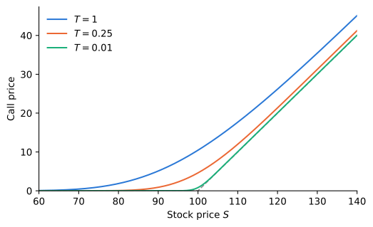
Example 5 A stock trades at S_{0} = 100, has volatility \sigma = 0.2, and the risk-free rate is r = 0.05. For options with strike K = 100 and maturity T = 1 year, d_{1} = \frac{\ln(100 / 100) + (0.05 + 0.5 \times 0.2^{2}) \times 1}{0.2 \sqrt{1}} = 0.35, \qquad d_{2} = d_{1} - \sigma \sqrt{T} = 0.15. The call is worth C = 100 N(0.35) - 100 e^{-0.05} N(0.15) = 10.45, and put-call parity gives the put price P = C - 100 + 100 e^{-0.05} = 5.57. The expected return \mu of the stock does not appear anywhere in the calculation.
Partial Differential Equations in the Black-Scholes Model
The Black-Scholes formula was originally derived as the solution of a partial differential equation (PDE). It is indeed the case that any derivative in the Black-Scholes model must satisfy the same PDE. Consider a derivative V that pays f(S_{T}) at time T.
If V is a function of S and t, then Itô’s lemma implies that \begin{aligned} \mathop{}\!\mathrm{d}V & = \frac{\partial V}{\partial S} \mathop{}\!\mathrm{d}S+ \frac{1}{2} \frac{\partial^{2} V}{\partial S^{2}} (\mathop{}\!\mathrm{d}S)^{2} + \frac{\partial V}{\partial t} \mathop{}\!\mathrm{d}t\\ & = \left( r S \frac{\partial V}{\partial S} + \frac{1}{2} \sigma^{2} S^{2} \frac{\partial^{2} V}{\partial S^{2}} + \frac{\partial V}{\partial t} \right) \mathop{}\!\mathrm{d}t+ \sigma S \frac{\partial V}{\partial S} \mathop{}\!\mathrm{d}B^{*}, \end{aligned} where we used the risk-neutral dynamics of S and (\mathop{}\!\mathrm{d}S)^{2} = \sigma^{2} S^{2} \mathop{}\!\mathrm{d}t. Equation (3) says that the drift of V under \operatorname{P}^{*} must be r V. Matching the drifts, any derivative written on S must satisfy the partial differential equation r S \frac{\partial V}{\partial S} + \frac{1}{2} \sigma^{2} S^{2} \frac{\partial^{2} V}{\partial S^{2}} + \frac{\partial V}{\partial t} = r V, \tag{6} with the terminal condition V(S, T) = f(S). Different derivatives satisfy the same equation and differ only in their terminal conditions. The expected return \mu does not appear, for the same reason that it does not appear in the Black-Scholes formula.
The diffusion term also has an interpretation. The derivative has volatility \sigma S \, \partial V / \partial S and is driven by the same Brownian motion as the stock, so a portfolio that holds the derivative and sells \partial V / \partial S shares of the stock has no exposure to \mathop{}\!\mathrm{d}B. This number of shares is the delta of the derivative. A riskless portfolio must earn the risk-free rate, which gives the same equation (6) and was the original argument of Black and Scholes.
It is in theory possible to solve the partial differential equation subject to a terminal value to price any derivative like a European call or put option written on the stock. In practice, it is easier to use a change of measure to find the value of the derivative. The two approaches are connected: the solution of (6) is the risk-neutral expectation (4), a link known as the Feynman-Kac formula.