Modeling Stock Prices
A Brownian motion can take any value, positive or negative, and its changes over a period do not depend on its level. Neither property fits a stock price. Prices cannot fall below zero, and a stock trading at $200 typically moves by about twice as many dollars in a day as the same stock trading at $100. What stays roughly stable over time is the distribution of returns, the percentage changes in price. The standard model therefore lets returns, not price changes, follow a Brownian motion with drift. The resulting process is called a geometric Brownian motion, and it is the model of stock prices behind the Black-Scholes formula.
These notes apply the tools of the notes on stochastic calculus to this model. Itô’s formula solves for the stock price explicitly, which shows that the price is lognormally distributed. We then compute its moments, explain why the expected return of a stock is higher than the growth rate of its price, and derive the dynamics of functions of the stock price, which is the step that leads to option pricing. These notes draw on Shreve (2004).
Geometric Brownian Motion
Over a short interval of length \Delta t, suppose the return on the stock is \frac{\Delta S_{t}}{S_{t}} = \mu \Delta t + \sigma \Delta B_{t}, which is normally distributed with mean \mu \Delta t and variance \sigma^{2} \Delta t. Letting \Delta t \to 0 gives the stochastic differential equation \frac{\mathop{}\!\mathrm{d}S_{t}}{S_{t}} = \mu \mathop{}\!\mathrm{d}t+ \sigma \mathop{}\!\mathrm{d}B_{t}, \qquad \text{or} \qquad \mathop{}\!\mathrm{d}S_{t} = \mu S_{t} \mathop{}\!\mathrm{d}t+ \sigma S_{t} \mathop{}\!\mathrm{d}B_{t}. \tag{1} The process \{S_{t}\} is a geometric Brownian motion (GBM).1 It is an Itô process whose drift \mu S_{t} and diffusion coefficient \sigma S_{t} are proportional to the price. The constant \mu is the expected return of the stock per unit of time, and \sigma is the volatility of its returns. Both are usually quoted per year.
1 A common criticism of this model is that volatility is not constant and that prices sometimes jump. The criticism is right about the data but not about the method. Nothing in the tools of these notes requires constant coefficients. Letting the variance follow its own Itô process gives a stochastic volatility model such as that of Heston (1993), and adding a Poisson process gives the jump models in the notes on pricing with jumps. Geometric Brownian motion is the simplest member of this family, which is why we start with it.
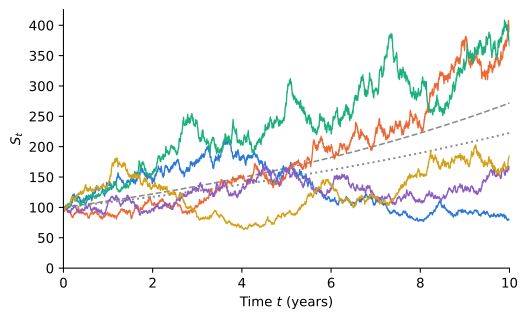
Figure 1 shows five simulated paths with S_{0} = 100, \mu = 0.10, and \sigma = 0.20 over ten years. Unlike a Brownian motion, the paths never fall below zero, and their fluctuations grow with the price level: a path that has doubled moves by about twice as many dollars as it did at the start. The paths also fan out over time, and they spread unevenly, with a few ending far above the rest. This skewness is why the expected price, the dashed line, sits above the median price, the dotted line, a gap we explain later in these notes.
Solving for the Stock Price
The logarithm of the price turns returns into additive changes, so we apply Itô’s lemma to X_{t} = \ln S_{t}. With f(S) = \ln S, the derivatives are f'(S) = 1 / S and f''(S) = -1 / S^{2}, and the multiplication table gives (\mathop{}\!\mathrm{d}S_{t})^{2} = \sigma^{2} S_{t}^{2} \mathop{}\!\mathrm{d}t. Therefore, \begin{aligned} \mathop{}\!\mathrm{d}X_{t} & = \frac{1}{S_{t}} \mathop{}\!\mathrm{d}S_{t} + \frac{1}{2} \left(-\frac{1}{S_{t}^{2}}\right) (\mathop{}\!\mathrm{d}S_{t})^{2} \\ & = \mu \mathop{}\!\mathrm{d}t+ \sigma \mathop{}\!\mathrm{d}B_{t} - \frac{1}{2} \sigma^{2} \mathop{}\!\mathrm{d}t\\ & = \left(\mu - \tfrac{1}{2} \sigma^{2}\right) \mathop{}\!\mathrm{d}t+ \sigma \mathop{}\!\mathrm{d}B_{t}. \end{aligned} The right-hand side has constant coefficients, so the log price is a Brownian motion with drift. Integrating from 0 to T gives X_{T} - X_{0} = \left(\mu - \frac{1}{2} \sigma^{2}\right) T + \sigma B_{T}, and taking exponentials, S_{T} = S_{0} \exp\left(\left(\mu - \tfrac{1}{2} \sigma^{2}\right) T + \sigma B_{T}\right). \tag{2}
The term -\frac{1}{2} \sigma^{2} is the Itô correction. Without it, ordinary calculus would suggest \mathop{}\!\mathrm{d}\ln S_{t} = \mathop{}\!\mathrm{d}S_{t} / S_{t} and a log price with drift \mu.
We can confirm the solution in a second way. Writing (2) as S_{t} = S_{0} e^{\mu t} Z_{t}, \qquad Z_{t} = \exp\left(\sigma B_{t} - \tfrac{1}{2} \sigma^{2} t\right), shows that the stock price is a deterministic exponential growth path times the exponential martingale from the notes on stochastic calculus, which satisfies \mathop{}\!\mathrm{d}Z_{t} = \sigma Z_{t} \mathop{}\!\mathrm{d}B_{t}. Since e^{\mu t} has no diffusion term, the product rule gives \mathop{}\!\mathrm{d}S_{t} = S_{0} \left(\mu e^{\mu t} Z_{t} \mathop{}\!\mathrm{d}t+ e^{\mu t} \sigma Z_{t} \mathop{}\!\mathrm{d}B_{t}\right) = \mu S_{t} \mathop{}\!\mathrm{d}t+ \sigma S_{t} \mathop{}\!\mathrm{d}B_{t}, which is (1).
The Distribution of the Stock Price
Since B_{T} \sim \mathcal{N}(0, T), equation (2) implies that the log price is normally distributed, \ln S_{T} \sim \mathcal{N}\left(\ln S_{0} + \left(\mu - \tfrac{1}{2} \sigma^{2}\right) T, \, \sigma^{2} T\right). In other words, S_{T} has a lognormal distribution, as defined in the notes on continuous distributions. The price is always positive, and the continuously compounded return \ln(S_{T} / S_{0}) over a horizon T is normal with mean \left(\mu - \frac{1}{2} \sigma^{2}\right) T and standard deviation \sigma \sqrt{T}. Probabilities about the stock price can be computed by translating them into statements about this normal return.
Example 1 A stock that follows a GBM has an expected return of 12% per year and a volatility of 25% per year, and its current price is $25. Over T = 0.5 years, the log price X_{T} = \ln S_{T} has \begin{aligned} \operatorname{E}(X_{T}) & = \ln(25) + \left(0.12 - 0.5 (0.25)^{2}\right)(0.5) = 3.2633, \\ \operatorname{SD}(X_{T}) & = 0.25 \sqrt{0.5} = 0.1768. \end{aligned} A 95% probability interval for X_{T} is 3.2633 \pm 1.96 (0.1768), and exponentiating its endpoints gives \left[e^{3.2633 - 1.96 (0.1768)}, e^{3.2633 + 1.96 (0.1768)}\right] = [18.48, 36.96]. There is a 95% probability that the stock price in six months will lie between $18.48 and $36.96. The interval is not symmetric around the current price, because a lognormal distribution is skewed to the right.
Moments of the Stock Price
The process S_{t} e^{-\mu t} = S_{0} Z_{t} is a martingale, so its expectation stays at S_{0}, and therefore \operatorname{E}(S_{T}) = S_{0} e^{\mu T}. The expected stock price grows at the rate \mu, which is why \mu is the expected return. The second moment follows from the normal MGF. Since S_{T}^{2} = S_{0}^{2} \exp\left((2 \mu - \sigma^{2}) T + 2 \sigma B_{T}\right) and \operatorname{E}(e^{2 \sigma B_{T}}) = e^{2 \sigma^{2} T}, \operatorname{E}(S_{T}^{2}) = S_{0}^{2} e^{(2 \mu + \sigma^{2}) T} = \operatorname{E}(S_{T})^{2} e^{\sigma^{2} T}.
The standard deviation is proportional to the expected price and, at long horizons, grows at the exponential rate \frac{1}{2} \sigma^{2} on top of the growth of the mean, so the uncertainty about the future price grows much faster than the expected price.
Example 2 For the stock in Example 1, the expected price and the standard deviation of the price six months from now are \begin{aligned} \operatorname{E}(S_{T}) & = 25 e^{0.12 (0.5)} = \$26.55, \\ \operatorname{SD}(S_{T}) & = 26.55 \sqrt{e^{0.25^{2} (0.5)} - 1} = \$4.73. \end{aligned}
Expected Return and Growth Rate
The log price grows at the rate \mu - \frac{1}{2} \sigma^{2}, while the expected price grows at the faster rate \mu. Both statements are correct, and the gap between them is a consequence of the skewness of the lognormal distribution. The median of S_{T} is the price at which the normal log price is at its mean, \text{Median}(S_{T}) = S_{0} e^{\left(\mu - \frac{1}{2} \sigma^{2}\right) T} < S_{0} e^{\mu T} = \operatorname{E}(S_{T}). Half of the paths end below the median, and more than half end below the mean. A few paths that end very high pull the mean above what a typical path achieves, as Figure 1 shows. The rate \mu - \frac{1}{2} \sigma^{2} is the growth rate that an investor holding the stock for a long time will typically realize, since the realized growth rate \frac{1}{T} \ln(S_{T} / S_{0}) converges to it as T \to \infty, and the expected return \mu is the rate at which wealth grows on average across all paths.
Example 3 A stock has an expected return of \mu = 0.1 and a volatility of \sigma = 0.2. Its log price grows at the rate 0.1 - 0.5 \times 0.2^{2} = 0.08 per year. Over T = 10 years, the expected price is e^{0.1 \times 10} = 2.72 times the current price, but the median price is only e^{0.08 \times 10} = 2.23 times the current price. The stock ends below its expected price when \sigma B_{T} < \frac{1}{2} \sigma^{2} T, which has probability \operatorname{P}\left(Z < \tfrac{1}{2} \sigma \sqrt{T}\right) = \operatorname{P}\left(Z < 0.3162\right) = 0.6241, where Z is a standard normal random variable.
The same distinction applies to the example on hitting a barrier in the notes on Brownian motion. There, the logarithm of the endowment’s value had drift 0.04 and volatility 0.15. If its value follows a GBM, that drift is \mu - \frac{1}{2} \sigma^{2} in the notation of these notes, so the expected return is \mu = 0.04 + \frac{1}{2} (0.15)^{2} = 0.05125.
Functions of the Stock Price
A derivative written on the stock, such as an option, has a price that depends on the current stock price and on time. If X_{t} = f(S_{t}, t), Itô’s lemma from the notes on stochastic calculus gives \mathop{}\!\mathrm{d}X_{t} = \frac{\partial f}{\partial S} \mathop{}\!\mathrm{d}S_{t} + \frac{1}{2} \frac{\partial^{2} f}{\partial S^{2}} (\mathop{}\!\mathrm{d}S_{t})^{2} + \frac{\partial f}{\partial t} \mathop{}\!\mathrm{d}t, and substituting (1) and (\mathop{}\!\mathrm{d}S_{t})^{2} = \sigma^{2} S_{t}^{2} \mathop{}\!\mathrm{d}t, \mathop{}\!\mathrm{d}X_{t} = \left(\mu S_{t} \frac{\partial f}{\partial S} + \frac{1}{2} \sigma^{2} S_{t}^{2} \frac{\partial^{2} f}{\partial S^{2}} + \frac{\partial f}{\partial t}\right) \mathop{}\!\mathrm{d}t+ \sigma S_{t} \frac{\partial f}{\partial S} \mathop{}\!\mathrm{d}B_{t}. \tag{3} The function X_{t} is driven by the same Brownian motion as the stock, with a volatility that depends on the sensitivity \partial f / \partial S of X to the stock price. This common source of risk is what allows an option to be replicated with the stock and is the starting point for the notes on derivatives pricing.
For notational simplicity, I like to write X_{S} = \partial f / \partial S and X_{SS} = \partial^{2} f / \partial S^{2}. An option that expires at a fixed date T is often more conveniently written as a function of the time to maturity \tau = T - t than of calendar time. As calendar time moves forward by \mathop{}\!\mathrm{d}t, the time to maturity decreases by \mathop{}\!\mathrm{d}t, so that \partial f / \partial t = -\partial f / \partial \tau. Writing X_{\tau} = \partial f / \partial \tau, Itô’s lemma becomes \mathop{}\!\mathrm{d}X = X_{S} \mathop{}\!\mathrm{d}S + \frac{1}{2} X_{SS} (\mathop{}\!\mathrm{d}S)^{2} - X_{\tau} \mathop{}\!\mathrm{d}t.
Example 4 Let X_{t} = S_{t}^{a} for a constant a. Then X_{S} = a S^{a - 1} and X_{SS} = a (a - 1) S^{a - 2}, and (3) gives \frac{\mathop{}\!\mathrm{d}X_{t}}{X_{t}} = \left(a \mu + \tfrac{1}{2} a (a - 1) \sigma^{2}\right) \mathop{}\!\mathrm{d}t+ a \sigma \mathop{}\!\mathrm{d}B_{t}. A power of a GBM is again a GBM, with volatility |a| \sigma. For a = 2, the expected growth rate of S_{t}^{2} is 2 \mu + \sigma^{2}, which matches the second moment computed above.
Example 5 Let S_{t} be the price of one euro in dollars and suppose it follows a GBM with expected rate of change \mu and volatility \sigma. The price of one dollar in euros is 1 / S_{t}, and Example 4 with a = -1 gives \frac{\mathop{}\!\mathrm{d}(1 / S_{t})}{1 / S_{t}} = \left(-\mu + \sigma^{2}\right) \mathop{}\!\mathrm{d}t- \sigma \mathop{}\!\mathrm{d}B_{t}. If the dollar price of the euro is expected to stay flat, \mu = 0, the euro price of the dollar is still expected to rise at the rate \sigma^{2}. If 0 < \mu < \sigma^{2}, each currency is expected to appreciate against the other at the same time. This puzzle, known as Siegel’s paradox, is resolved by noting that expected rates of change are measured in different units, and it is a direct consequence of the Itô correction.