Problem Set 4 Solutions
Investment Theory
Problem 1
- If you use the CAPM as your asset pricing model, can a stock have a positive alpha but a Sharpe ratio lower than the market? How can this be possible?
- Why do we claim that a stock with a negative alpha is considered overpriced?
- Can a risky financial asset have no firm-specific risk? If so, give an example of such an asset.
- In the group project, you maximized the Sharpe ratio of a portfolio of sector ETFs with and without short sales. Why can the short-sale constrained portfolio never have a higher Sharpe ratio than the unconstrained one in the sample used to estimate the inputs? Why might it nevertheless perform better out of sample?
Solution.
- Yes. Alpha measures the expected return of a stock relative to what the CAPM requires for its beta, and beta reflects only systematic risk. The Sharpe ratio divides the risk premium by total volatility, which also includes firm-specific risk. A stock with a lot of firm-specific risk can therefore beat the CAPM and still have a low Sharpe ratio. For example, with r_f = 4\%, \operatorname{E}(r_M) = 10\% and \sigma_M = 20\%, a stock with \beta = 1, \alpha = 1\% and \sigma = 50\% has a Sharpe ratio of 7\% / 50\% = 0.14, against 0.30 for the market. The firm-specific risk is not a problem for a diversified investor, who can hold a small position in the stock and diversify most of that risk away.
- A negative alpha means the stock’s expected return is below what the CAPM requires for its systematic risk. Investors would rather hold a combination of the market and T-bills with the same beta, which offers a higher expected return, so they sell the stock. Selling pushes its price down, which raises its expected return, until the alpha disappears. A stock whose price has to fall to offer a fair expected return is overpriced today.
- Yes. An asset has no firm-specific risk when all of its risk is systematic, that is, when its returns are perfectly correlated with the market and its R-square is 1. A broadly diversified index fund that tracks the market portfolio is the standard example: it is risky, since its returns move with the market, but it carries no firm-specific risk because diversification has already removed it.
- Every long-only portfolio is also available when short sales are allowed, so the unconstrained optimizer can always choose the constrained solution. In the estimation sample, it can only do as well or better. Out of sample, the inputs are estimates, and the expected returns in particular contain a lot of noise. The unconstrained portfolio bets on that noise with large long and short positions, and those bets do not pay off on new data. The short-sale constraint rules out the most extreme of these positions, so the constrained portfolio often performs better out of sample.
Problem 2 The risk-free rate is 4%, and the market portfolio has an expected return of 10% with a standard deviation of 20%. Harbor Logistics stock has a return standard deviation of 40% and a correlation of 0.35 with the market. Harbor trades at $100 per share and is expected to pay a constant dividend in perpetuity.
- Compute the beta of Harbor stock and its expected return according to the CAPM.
- What fraction of the variance of Harbor’s returns is systematic? What is the standard deviation of its firm-specific returns?
- An analyst forecasts that Harbor will earn 12% over the coming year. Compute Harbor’s alpha given this forecast. According to the analyst, is the stock underpriced, overpriced, or fairly priced?
- Ignore the analyst’s forecast and assume that investors discount Harbor’s dividends at the CAPM expected return from part a, so that the price satisfies the perpetuity formula P = \frac{D}{\operatorname{E}(r)}. Compute the dividend that justifies the current price of $100. What would be the new price of Harbor stock if its correlation with the market doubled, with all other variables unchanged?
Solution.
- The beta of Harbor is \beta = \frac{\rho_{rM} \, \sigma(r)}{\sigma_M} = \frac{0.35 \times 0.40}{0.20} = 0.70, and its CAPM expected return is \operatorname{E}(r) = 4\% + 0.70 \times (10\% - 4\%) = 8.2\%.
- The systematic variance is \beta^2 \sigma_M^2 = 0.70^2 \times 0.20^2 = 0.0196, out of a total variance of 0.40^2 = 0.16, so the systematic fraction is 0.0196 / 0.16 = 12.25\%, which equals \rho_{rM}^2 = 0.35^2. The firm-specific variance is 0.16 - 0.0196 = 0.1404, so the firm-specific standard deviation is \sqrt{0.1404} = 37.47\%.
- Alpha is the forecast return minus the CAPM expected return: \alpha = 12\% - 8.2\% = 3.8\%. The analyst expects Harbor to earn more than the CAPM requires for its risk, so according to the analyst the stock is underpriced.
- The dividend that justifies the price is D = P \times \operatorname{E}(r) = 100 \times 0.082 = \$8.20. If the correlation doubles to 0.70, beta doubles to 0.70 \times 0.40 / 0.20 = 1.40 and the expected return becomes 4\% + 1.40 \times 6\% = 12.4\%. The new price is P = \frac{8.20}{0.124} = \$66.13. The stock’s total volatility is unchanged, but more of it is now systematic, so investors require a higher return and pay a lower price for the same dividends.
Problem 3 Consider the two (excess return) index-model regression results for stocks A and B:
| Stock | Alpha | Beta | Firm-Specific Standard Deviation |
|---|---|---|---|
| A | -0.5% | 1.4 | 10% |
| B | 2.5% | 0.6 | 23% |
The risk-free rate over the period was 5%, whereas the market’s average return was 12% with a standard deviation of 25%.
- Compute the expected return of stocks A and B.
- Compute the variance and standard deviation of stocks A and B.
- Compute the Sharpe ratio of stocks A and B.
- Compute the regression R-square of stocks A and B.
- Compute the covariance of returns between A and B.
- Suppose you form a portfolio P composed of 25% of A and 75% of B. Compute the expected return, beta, standard deviation and firm-specific standard deviation of portfolio P.
Solution. The market’s excess return is \operatorname{E}(R_M) = 12\% - 5\% = 7\% and its variance is \sigma_M^2 = 0.25^2 = 0.0625.
- The expected return is r_f + \alpha + \beta \operatorname{E}(R_M): \begin{aligned} \operatorname{E}(r_A) &= 5\% - 0.5\% + 1.4 \times 7\% = 14.3\%, \\ \operatorname{E}(r_B) &= 5\% + 2.5\% + 0.6 \times 7\% = 11.7\%. \end{aligned}
- The variance is \beta^2 \sigma_M^2 + \sigma^2(e): \begin{aligned} \sigma_A^2 &= 1.4^2 \times 0.0625 + 0.10^2 = 0.1225 + 0.0100 = 0.1325, & \sigma_A &= 36.40\%, \\ \sigma_B^2 &= 0.6^2 \times 0.0625 + 0.23^2 = 0.0225 + 0.0529 = 0.0754, & \sigma_B &= 27.46\%. \end{aligned}
- The Sharpe ratios are S_A = \frac{0.143 - 0.05}{0.3640} = 0.26, \qquad S_B = \frac{0.117 - 0.05}{0.2746} = 0.24.
- The R-square is the systematic share of the variance: R_A^2 = \frac{0.1225}{0.1325} = 0.92, \qquad R_B^2 = \frac{0.0225}{0.0754} = 0.30.
- In the index model, the covariance comes only through the market: \operatorname{Cov}(r_A, r_B) = \beta_A \beta_B \sigma_M^2 = 1.4 \times 0.6 \times 0.0625 = 0.0525.
- For portfolio P, \begin{aligned} \operatorname{E}(r_P) &= 0.25 \times 14.3\% + 0.75 \times 11.7\% = 12.35\%, \\ \beta_P &= 0.25 \times 1.4 + 0.75 \times 0.6 = 0.80, \\ \sigma^2(e_P) &= 0.25^2 \times 0.10^2 + 0.75^2 \times 0.23^2 = 0.000625 + 0.029756 = 0.030381, \\ \sigma_P^2 &= 0.80^2 \times 0.0625 + 0.030381 = 0.070381, \end{aligned} so the firm-specific standard deviation is \sigma(e_P) = 17.43\% and the standard deviation is \sigma_P = 26.53\%. The same variance follows from the two-asset formula, 0.25^2 \times 0.1325 + 0.75^2 \times 0.0754 + 2 \times 0.25 \times 0.75 \times 0.0525 = 0.070381.
Problem 4 A pension fund manager is considering three mutual funds. The first is a stock fund, the second is a long-term government and corporate bond fund, and the third is a T-bill money market fund. The statistical properties of the funds are as follows.
| Expected Return | Standard Deviation | |
|---|---|---|
| Stock Fund (S) | 15% | 25% |
| Bond Fund (B) | 8% | 15% |
| T-bill Fund (F) | 5% | 0% |
Analysts estimate that the maximum Sharpe ratio portfolio (Q) has an expected return of 20% and a standard deviation of 30%.
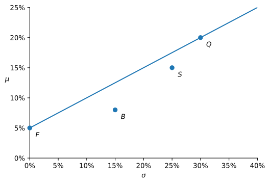
- In a μ-σ diagram, draw the capital allocation line (CAL) of Q, and indicate where the mutual funds S, B, and F are located. Which portfolios are efficient or inefficient? Why?
- Determine the weights of an efficient portfolio that has the same standard deviation as the stock fund (S). What’s the expected return of this portfolio?
- Determine the weights of an efficient portfolio that has the same expected return as the bond fund (B). What’s the standard deviation of this portfolio?
- The pension fund ranks portfolios using the utility function U = \mu - \frac{1}{2} A \sigma^{2} with A = 5. What fraction of the fund should be invested in Q, and what fraction in T-bills? Compute the expected return, standard deviation and certainty equivalent of this optimal portfolio, and compare it with the certainty equivalent of investing everything in the stock fund (S).
Solution.
- The capital allocation line of Q starts at r_f = 5\% with slope equal to the Sharpe ratio of Q, (20\% - 5\%)/30\% = 0.50. The Sharpe ratios of the stock and bond funds are (15\% - 5\%)/25\% = 0.40 and (8\% - 5\%)/15\% = 0.20, so both lie below the line (Figure 1) and are inefficient: a mix of Q and T-bills with the same volatility has a higher expected return. The efficient portfolios are those on the line. The T-bill fund is its starting point, so it is efficient, as is Q.
- A weight w in Q gives volatility w \times 30\%, so matching the stock fund requires w = 25/30 = 0.8333: 83.33% in Q and 16.67% in T-bills. The expected return is \mu = 5\% + 0.8333 \times (20\% - 5\%) = 17.5\%, 2.5 percentage points more than the stock fund at the same risk.
- Matching the bond fund’s 8% requires 5\% + w \times 15\% = 8\%, so w = 0.20: 20% in Q and 80% in T-bills. The standard deviation is 0.20 \times 30\% = 6\%, against 15% for the bond fund.
- The optimal fraction in Q is w^* = \frac{\mu_Q - r_f}{A \sigma_Q^2} = \frac{0.20 - 0.05}{5 \times 0.30^2} = \frac{0.15}{0.45} = 0.3333, so the fund invests one third in Q and two thirds in T-bills. The portfolio has \begin{aligned} \mu &= 5\% + 0.3333 \times 15\% = 10\%, \\ \sigma &= 0.3333 \times 30\% = 10\%, \\ U &= 0.10 - \tfrac{1}{2} \times 5 \times 0.10^2 = 0.075. \end{aligned} Its certainty equivalent is 7.5%. Investing everything in the stock fund gives 0.15 - \frac{1}{2} \times 5 \times 0.25^2 = -0.0063, a certainty equivalent of -0.63\%, worse even than the 5% of T-bills. The stock fund is both inefficient and far too risky for an investor with A = 5.
Problem 5 Next year the economy can be in one of three states. You forecast the following returns for two stocks, X and Y.
| State | Probability | Return on X | Return on Y |
|---|---|---|---|
| Boom | 0.3 | 28% | 4% |
| Normal | 0.4 | 12% | 18% |
| Recession | 0.3 | -8% | -2% |
- Compute the expected return and standard deviation of each stock.
- Compute the covariance and the correlation between the returns of X and Y.
- Compute the weights, expected return and standard deviation of the minimum-variance portfolio of X and Y.
- Compare the minimum-variance portfolio with stock Y. Would a mean-variance investor who can only invest in X and Y ever put all of her wealth in Y? Explain.
- The weights you found in part c depend only on the variances and the covariance of the two stocks, not on their expected returns. In the group project, you estimated both the maximum Sharpe ratio and the minimum variance portfolios from five years of monthly returns. Explain why not relying on expected returns can be an advantage of the minimum variance portfolio.
Solution.
- The expected returns are \begin{aligned} \operatorname{E}(r_X) &= 0.3 \times 28\% + 0.4 \times 12\% + 0.3 \times (-8\%) = 10.8\%, \\ \operatorname{E}(r_Y) &= 0.3 \times 4\% + 0.4 \times 18\% + 0.3 \times (-2\%) = 7.8\%, \end{aligned} and the variances are \begin{aligned} \operatorname{V}(r_X) &= 0.3 (0.172)^2 + 0.4 (0.012)^2 + 0.3 (-0.188)^2 = 0.019536, & \sigma_X &= 13.98\%, \\ \operatorname{V}(r_Y) &= 0.3 (-0.038)^2 + 0.4 (0.102)^2 + 0.3 (-0.098)^2 = 0.007476, & \sigma_Y &= 8.65\%. \end{aligned}
- The covariance is \begin{aligned} \operatorname{Cov}(r_X, r_Y) &= 0.3 (0.172)(-0.038) + 0.4 (0.012)(0.102) + 0.3 (-0.188)(-0.098) \\ &= -0.001961 + 0.000490 + 0.005527 = 0.004056, \end{aligned} and the correlation is 0.004056 / (0.1398 \times 0.0865) = 0.34.
- The minimum-variance weights are w_X = \frac{0.007476 - 0.004056}{0.019536 + 0.007476 - 2 \times 0.004056} = \frac{0.003420}{0.018900} = 0.1810, and w_Y = 0.8190. The portfolio has \begin{aligned} \operatorname{E}(r) &= 0.1810 \times 10.8\% + 0.8190 \times 7.8\% = 8.34\%, \\ \operatorname{V}(r) &= 0.1810^2 \times 0.019536 + 0.8190^2 \times 0.007476 \\ &\quad + 2 \times 0.1810 \times 0.8190 \times 0.004056 = 0.006857, \end{aligned} so its standard deviation is 8.28%.
- The minimum-variance portfolio has a higher expected return than Y (8.34% against 7.8%) and a lower standard deviation (8.28% against 8.65%). Y is dominated, so a mean-variance investor never puts all of her wealth in it, whatever her risk aversion: moving 18% of her wealth into X raises her expected return and lowers her risk at the same time.
- Expected returns are very hard to estimate. The standard error of an average return is the volatility divided by the square root of the number of years, so with five years of data and a volatility of 20% per year it is about 20\% / \sqrt{5} \approx 9\%, as large as the risk premiums being estimated. Variances and covariances are estimated far more precisely, because they improve with the number of observations, here 60 months, rather than with the length of the sample in years. The maximum Sharpe ratio weights are very sensitive to the estimated means and tilt heavily toward assets whose sample average happened to be high, which is often noise. The minimum variance portfolio uses only the better-estimated inputs, so its weights are more stable and its out-of-sample performance closer to what the sample suggests.
Problem 6 Two risky assets A and B have the following characteristics:
- \operatorname{E}(r_{A}) = 0.20, \sigma_{A} = 0.28
- \operatorname{E}(r_{B}) = 0.30, \sigma_{B} = 0.48
- \rho_{AB} = +1
- Compute the expected return of an asset with zero return variance.
- Suppose that in addition to A and B, there is a risk-free asset offering a return of 5%. Is there an arbitrage opportunity? If so, clearly explain how an investor could arbitrage this opportunity, and explain why this would be an arbitrage.
Solution.
- With \rho_{AB} = +1, the volatility of a portfolio is |w_A \sigma_A + w_B \sigma_B|, which is zero when w_A = \frac{\sigma_B}{\sigma_B - \sigma_A} = \frac{0.48}{0.48 - 0.28} = 2.4, \qquad w_B = -1.4. This portfolio has zero variance and expected return \operatorname{E}(r) = 2.4 \times 20\% - 1.4 \times 30\% = 6\%.
- Yes. The zero-variance portfolio earns a sure 6%, while the risk-free asset earns 5%. An investor borrows at 5% and invests the proceeds in the zero-variance portfolio: for each $1 borrowed, they buy $2.40 of A and short $1.40 of B, which costs exactly $1. At the end of the year the position is worth $1.06 for sure and the loan costs $1.05, leaving $0.01 per dollar borrowed. This is an arbitrage because the strategy needs no money down, has no risk, and pays a positive amount for sure; scaling it up scales the profit without limit.
Problem 7 You have a logarithmic utility function u(W) = \ln W and your current wealth is $10,000. There is a 10% probability that your wealth decreases to $1,000, and a 90% probability that your wealth remains at $10,000. You are considering two insurance policies:
- Plan A: Pays $5,000 if your wealth decreases to $1,000 and costs $500 upfront.
- Plan B: Pays $8,000 if your wealth decreases to $1,000 and costs $800 upfront.
Evaluate whether you should choose Plan A, Plan B, or opt not to purchase insurance. Provide a clear explanation of your decision.
Solution. The wealth in each case, net of the premium, is:
| Choice | Bad state (prob. 0.1) | Good state (prob. 0.9) |
|---|---|---|
| No insurance | $1,000 | $10,000 |
| Plan A | 1{,}000 + 5{,}000 - 500 = \$5{,}500 | 10{,}000 - 500 = \$9{,}500 |
| Plan B | 1{,}000 + 8{,}000 - 800 = \$8{,}200 | 10{,}000 - 800 = \$9{,}200 |
The expected utilities are \begin{aligned} \text{No insurance:} \quad & 0.1 \ln 1{,}000 + 0.9 \ln 10{,}000 = 8.9801, \\ \text{Plan A:} \quad & 0.1 \ln 5{,}500 + 0.9 \ln 9{,}500 = 9.1044, \\ \text{Plan B:} \quad & 0.1 \ln 8{,}200 + 0.9 \ln 9{,}200 = 9.1155, \end{aligned} with certainty equivalents of $7,943, $8,995 and $9,095. You should choose Plan B. Both plans are actuarially fair: each costs exactly its expected payout (0.1 \times 5{,}000 = 500 and 0.1 \times 8{,}000 = 800), so neither changes your expected wealth of $9,100. With a fair price, a risk-averse investor wants as much coverage as possible, and Plan B covers more of the loss.