Problem Set 2 Solutions
Investment Theory
Problem 1 Every January, Kestrel Wealth Partners publishes the capital-market forecasts its advisers must use for the year ahead. This year’s numbers are an expected return on the market portfolio of 10.5% with a volatility of 16%, and a risk-free rate of 2.5%. Every portfolio the firm recommends mixes the market portfolio with T-bills, and clients may borrow at the risk-free rate, so all such portfolios lie on the capital market line.
- What is the Sharpe ratio of the market portfolio under these forecasts?
- Linda wants her portfolio to have a volatility of 12%. What fraction of her wealth should she hold in the market portfolio, and what expected return can the firm offer her?
- A second client, Desmond, wants an expected return of 11.5%. What position in the market portfolio does that require, and what volatility does it carry? Interpret the weight you obtain and explain what Desmond must do to achieve it.
Solution.
- The Sharpe ratio of the market portfolio is S_M = \frac{\operatorname{E}[r_M] - r_f}{\sigma_M} = \frac{0.105 - 0.025}{0.16} = 0.50.
- A portfolio with weight y in the market has volatility y \sigma_M, so Linda needs y = \frac{0.12}{0.16} = 0.75, that is, 75% in the market portfolio and 25% in T-bills. Her expected return is \operatorname{E}[r_P] = r_f + y (\operatorname{E}[r_M] - r_f) = 0.025 + 0.75 \times 0.08 = 8.5\%, which is also 2.5\% + 0.50 \times 12\% along the capital market line.
- Desmond needs y = \frac{0.115 - 0.025}{0.105 - 0.025} = 1.125, with volatility 1.125 \times 16\% = 18\%. A weight above one means he invests 112.5% of his wealth in the market portfolio and -12.5\% in T-bills: he borrows 12.5% of his wealth at the risk-free rate and puts the borrowed money in the market along with his own. Leverage scales the market’s risk premium and volatility by the same factor, 1.125: the risk premium rises from 8% to 9% and the volatility from 16% to 18%.
Problem 2 Two clients of the same advisory firm complete the identical risk questionnaire. Thomas scores a risk-aversion coefficient of A = 2, while Edith scores A = 6. Both are shown the same balanced fund, which the firm forecasts will earn an expected return of 11% with a volatility of 20%. T-bills currently yield 2.5%. Both clients rank portfolios using the utility function U = \mu - 0.5 A \sigma^{2}, where \mu and \sigma are expressed as decimals rather than percentages.
- Compute each client’s utility score for the balanced fund, and interpret the two numbers as certainty equivalents.
- If each client had to choose between the balanced fund and T-bills alone, what would each one do? Explain why the same fund can be attractive to one investor and unattractive to the other.
- Edith is currently indifferent between the portfolio she already owns (which is not the balanced fund) and a sure return of 4%. What expected return would a portfolio with a volatility of 10% have to offer for her to be just as well off holding it instead?
Solution.
- With \mu = 0.11 and \sigma^2 = 0.04, \begin{aligned} U_{\text{Thomas}} &= 0.11 - 0.5 \times 2 \times 0.04 = 0.07, \\ U_{\text{Edith}} &= 0.11 - 0.5 \times 6 \times 0.04 = -0.01. \end{aligned} A utility score is the certainty equivalent rate: the sure return that the investor values as much as the risky fund. Thomas values the fund like a sure 7%, while Edith values it like a sure loss of 1%.
- T-bills offer a sure 2.5%, so their utility score is 2.5% for both. Thomas prefers the fund, since 7\% > 2.5\%, and Edith prefers T-bills, since -1\% < 2.5\%. Both see the same expected return and volatility, but the penalty for risk, 0.5 A \sigma^2, is three times larger for Edith: 12 percentage points against 4. The 8.5% risk premium of the fund more than compensates Thomas for its risk but not Edith.
- Her current portfolio is worth a utility of 0.04 to her. A portfolio with \sigma = 0.10 gives her the same utility if \mu - 0.5 \times 6 \times 0.10^2 = 0.04 \quad\Longrightarrow\quad \mu = 0.04 + 0.03 = 7\%.
Problem 3 You run a boutique fund whose returns you forecast at 14% per year with a volatility of 25% per year. Your clients can also invest in T-bills, which yield 4% per year. Each client chooses the mix of your fund and T-bills that maximizes U = \mu - 0.5 A \sigma^{2}, where A is the client’s risk-aversion coefficient.
- Your first client, Harold, has a risk-aversion coefficient of A = 3. What fraction of his wealth should he place in your fund?
- What are the expected return and volatility of Harold’s optimal portfolio, and what utility score does it deliver?
- A second client, Ingrid, is twice as risk-averse as Harold, with A = 6. Before computing anything, use the formula for the optimal weight to predict how her allocation to your fund should compare with Harold’s. Then verify your prediction.
Solution.
- The optimal weight in the risky fund is y^* = \frac{\operatorname{E}[r_P] - r_f}{A \sigma_P^2} = \frac{0.14 - 0.04}{3 \times 0.25^2} = \frac{0.10}{0.1875} = 0.5333, so Harold places 53.33% of his wealth in your fund and 46.67% in T-bills.
- His portfolio has \begin{aligned} \operatorname{E}[r_C] &= 0.04 + 0.5333 \times 0.10 = 9.33\%, \\ \sigma_C &= 0.5333 \times 0.25 = 13.33\%, \\ U &= 0.0933 - 0.5 \times 3 \times 0.1333^2 = 0.0667, \end{aligned} so the portfolio is worth a sure 6.67% to Harold, more than the 4% he could earn in T-bills alone.
- The optimal weight is inversely proportional to A, so doubling risk aversion should halve the allocation, to about 26.67%. Indeed, y^* = \frac{0.10}{6 \times 0.25^2} = \frac{0.10}{0.375} = 0.2667. Ingrid holds the same risky fund as Harold, only less of it.
Problem 4 Sitting down with a new client, an adviser sketches the picture below. The client has only two things to invest in: a savings account paying a certain 4%, marked F on the sketch, and a single risky asset B that the firm forecasts will earn 12% with a volatility of 20%. Every portfolio the client can build from the two lies on the straight line joining F and B.
The four curves are the client’s own indifference curves, drawn from the utility function U = \mu - 0.5 A \sigma^{2} and numbered so that a higher number means a happier client. Curve 1 cuts the straight line, curve 2 grazes it exactly once at the point marked P, and curves 3 and 4 float above it without ever making contact. The points C and D both lie on curve 4.
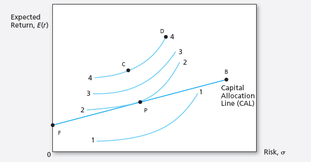
- How does the client rank C against D? Why can she not simply aim for one of them? Which of the four curves is the best she can actually reach, and what should the adviser say about each of the other three?
- The adviser eventually recommends putting half of the client’s wealth into B, which is the portfolio marked P in the sketch. For that recommendation to be the utility-maximizing one, what risk-aversion coefficient must the client have?
Solution.
- C and D lie on the same indifference curve, so the client is indifferent between them: D offers a higher expected return, which just compensates her for its higher risk. She cannot aim for either because curve 4 lies entirely above the line joining F and B, and every portfolio she can build lies on that line. The best curve she can reach is curve 2, at the tangency point P. Curve 1 is attainable, since it cuts the line, but every portfolio on it is worse than P, so the adviser should tell her she can do better. Curves 3 and 4 would make her happier, but no portfolio built from F and B reaches them, so the adviser should tell her they are out of reach.
- With the optimal weight y^* = (\operatorname{E}[r_B] - r_f)/(A \sigma_B^2) equal to 0.5, 0.5 = \frac{0.12 - 0.04}{A \times 0.20^2} = \frac{0.08}{0.04 A} \quad\Longrightarrow\quad A = 4.
Problem 5 You manage a risky fund with an expected return of 15% and a volatility of 24%. T-bills yield 3%. Your client, Ravi, puts 60% of his savings in your fund and the remaining 40% in a T-bill money market account.
What are the expected return and volatility of Ravi’s overall portfolio?
Your fund holds only three stocks, in the following proportions:
Asset Proportions Stock A 30% Stock B 45% Stock C 25% Looking through the fund to the underlying stocks, what are the investment proportions of Ravi’s overall portfolio, including his position in T-bills? Verify that they sum to 100%.
Compute the Sharpe ratio of your fund and the Sharpe ratio of Ravi’s overall portfolio. Ravi worries that holding 40% in T-bills has cost him in risk-adjusted terms. Is he right? Explain what your answer implies about which decision actually determines an investor’s reward-to-risk ratio.
Solution.
- Ravi’s portfolio has \begin{aligned} \operatorname{E}[r_C] &= 0.03 + 0.6 \times (0.15 - 0.03) = 10.2\%, \\ \sigma_C &= 0.6 \times 0.24 = 14.4\%. \end{aligned}
- Each stock’s share of Ravi’s wealth is 60% times its share of the fund: \begin{aligned} \text{Stock A} &: 0.60 \times 30\% = 18\%, \\ \text{Stock B} &: 0.60 \times 45\% = 27\%, \\ \text{Stock C} &: 0.60 \times 25\% = 15\%, \end{aligned} and T-bills are the remaining 40%. The proportions sum to 40\% + 18\% + 27\% + 15\% = 100\%.
- The Sharpe ratios are S_P = \frac{0.15 - 0.03}{0.24} = 0.50, \qquad S_C = \frac{0.102 - 0.03}{0.144} = 0.50. Ravi is wrong: holding T-bills scales the risk premium and the volatility by the same factor, 0.6, so the ratio is unchanged. Every mix of the fund and T-bills lies on the same capital allocation line, whose slope is the Sharpe ratio of the fund. The reward-to-risk ratio is set by the choice of the risky portfolio; how much to put in it only chooses a point on the line, according to the investor’s risk aversion.
Problem 6 The investment committee of a small college endowment is choosing between two managers. The Cascade Fund is the steadier of the two, with a forecast expected return of 10% and a volatility of 16%. The Ridgeline Fund is more aggressive, with an expected return of 17% and a volatility of 28%. What caught the committee’s attention is that the two funds tend to move against each other: the correlation between their returns is -0.15.
- One member proposes splitting the endowment evenly between the two funds. What expected return and volatility would that portfolio have?
- Another member argues the committee should instead find the combination of the two funds with the smallest possible volatility. Find the weights of that portfolio, and compute its expected return and volatility.
- Compare the volatilities you found in parts a and b with the volatility of each fund on its own. What makes it possible for even the simple 50/50 split to be less volatile than either fund held alone?
Solution. The covariance between the two funds is \sigma_{CR} = -0.15 \times 0.16 \times 0.28 = -0.00672.
- For the 50/50 split, \begin{aligned} \operatorname{E}[r_P] &= 0.5 \times 10\% + 0.5 \times 17\% = 13.5\%, \\ \sigma_P^2 &= 0.5^2 \times 0.16^2 + 0.5^2 \times 0.28^2 + 2 \times 0.5 \times 0.5 \times (-0.00672) \\ &= 0.0064 + 0.0196 - 0.00336 = 0.02264, \end{aligned} so \sigma_P = 15.05\%.
- The weight in Cascade that minimizes variance is w_C = \frac{\sigma_R^2 - \sigma_{CR}}{\sigma_C^2 + \sigma_R^2 - 2 \sigma_{CR}} = \frac{0.0784 + 0.00672}{0.0256 + 0.0784 + 0.01344} = \frac{0.08512}{0.11744} = 0.7248, so the portfolio holds 72.48% in Cascade and 27.52% in Ridgeline. Its expected return and variance are \begin{aligned} \operatorname{E}[r_{\min}] &= 0.7248 \times 10\% + 0.2752 \times 17\% = 11.93\%, \\ \sigma_{\min}^2 &= 0.7248^2 \times 0.0256 + 0.2752^2 \times 0.0784 + 2 \times 0.7248 \times 0.2752 \times (-0.00672) \\ &= 0.01671, \end{aligned} so \sigma_{\min} = 12.92\%.
- Both portfolios are less volatile than either fund alone: 15.05% and 12.92%, against 16% for Cascade and 28% for Ridgeline. The 50/50 split gets below Cascade because of the covariance term in its variance, 2 \times 0.5 \times 0.5 \times \sigma_{CR} = -0.00336. Both funds are held long and their returns tend to move in opposite directions, so this term is negative and lowers the variance from 0.026 to 0.02264. Without it, the split would have a volatility of 16.12%, slightly above that of Cascade.
Problem 7 A quantitative research team is studying how far diversification can go. The stocks in their universe each have a return variance of 0.25, and the average covariance between any two of them is 0.04. The team builds equally-weighted portfolios from this universe.
- What is the volatility of an equally-weighted portfolio of 20 of these stocks?
- What volatility does the equally-weighted portfolio approach as the number of stocks grows without bound?
- Interpret the limit you found in part b. What risk is the investor left holding after diversifying as much as possible, and why does that risk not disappear?
Solution.
- An equally-weighted portfolio of n stocks has variance \sigma_P^2 = \frac{1}{n} \bar{\sigma}^2 + \frac{n - 1}{n} \overline{\operatorname{Cov}}. With n = 20, \sigma_P^2 = \frac{0.25}{20} + \frac{19}{20} \times 0.04 = 0.0125 + 0.038 = 0.0505, so \sigma_P = 22.47\%, against 50% for a single stock.
- As n \to \infty, the first term vanishes and the second tends to the average covariance, so \sigma_P \to \sqrt{0.04} = 20\%.
- The limit is systematic, or market, risk. Each stock’s own risk, the part not shared with the others, averages out as the number of stocks grows, and that is what the first term captures. The covariance term does not vanish because it measures what the stocks have in common: they all respond to the same economy-wide shocks (business cycle, interest rates, inflation), and adding more stocks that respond to the same shocks cannot average them away. This is the risk investors must bear and the one that markets compensate.
Problem 8 Camila has $4,500,000 invested in a fully diversified portfolio that her adviser forecasts will earn 7.5% per year with a volatility of 11%. Her employer, Northwind Materials, has just vested $1,500,000 of company stock in her name, bringing her total wealth to $6,000,000. Her adviser forecasts that Northwind stock will earn 16% per year with a volatility of 30%, and estimates a correlation of 0.20 between Northwind stock and Camila’s diversified portfolio. T-bills yield 3.5%.
- Suppose Camila keeps the Northwind shares. What are the expected return and volatility of her new $6,000,000 portfolio?
- Suppose instead she sells the shares and puts the entire $1,500,000 into T-bills. What are the expected return and volatility of that portfolio?
- Selling the shares lowers both Camila’s expected return and her volatility. Which of the two portfolios should she prefer? Explain what the answer depends on.
- A colleague suggests a third option: sell the Northwind shares and use the $1,500,000 to buy stock in Sable Chemical, which the adviser forecasts will have exactly the same expected return and volatility as Northwind. The colleague argues that “it makes no difference whether she keeps Northwind or switches to Sable.” Is the colleague right? Justify your answer.
Solution.
- Northwind is 1.5/6 = 25\% of her wealth and the diversified portfolio 75%. The covariance is 0.20 \times 0.11 \times 0.30 = 0.0066, so \begin{aligned} \operatorname{E}[r] &= 0.75 \times 7.5\% + 0.25 \times 16\% = 9.625\%, \\ \sigma^2 &= 0.75^2 \times 0.11^2 + 0.25^2 \times 0.30^2 + 2 \times 0.75 \times 0.25 \times 0.0066 \\ &= 0.006806 + 0.005625 + 0.002475 = 0.014906, \end{aligned} and \sigma = 12.21\%.
- T-bills have no risk, so \begin{aligned} \operatorname{E}[r] &= 0.75 \times 7.5\% + 0.25 \times 3.5\% = 6.5\%, \\ \sigma &= 0.75 \times 11\% = 8.25\%. \end{aligned}
- It depends on her risk aversion. With U = \mu - 0.5 A \sigma^2, the two portfolios give equal utility when 0.09625 - 0.5 A \times 0.014906 = 0.065 - 0.5 A \times 0.006806 \quad\Longrightarrow\quad A = 7.72, so she should keep the shares if her A is below 7.72 and sell them for T-bills if it is above.
- The colleague is wrong. The risk of her total portfolio depends not only on the volatility of the stock she adds but also on its covariance with what she already holds, and the adviser has given no correlation between Sable and her diversified portfolio. With a lower correlation than 0.20, switching to Sable would lower her volatility at the same expected return; with a higher one, it would raise it. There is also a reason to prefer Sable that the numbers here leave out: Camila’s salary and job already depend on Northwind, so holding its stock ties her financial wealth to the same company as her income.