Problem Set 3 Solutions

Investment Theory

Problem 1 Suppose that there are many stocks in the security market and that the characteristics of stocks A and B are given as follows:

Stock	Expected Return	Standard Deviation
A	10%	5%
B	15%	10%

The correlation between the stock returns is -1. Suppose that it is possible to invest and borrow at the risk-free rate, r_{f}. What must be the value of the risk-free rate?

Solution. With a correlation of -1, a portfolio of A and B can be made riskless. Its volatility is |w_A \sigma_A - w_B \sigma_B|, which is zero when w_A \sigma_A = (1 - w_A) \sigma_B: w_A = \frac{\sigma_B}{\sigma_A + \sigma_B} = \frac{0.10}{0.05 + 0.10} = \frac{2}{3}, \qquad w_B = \frac{1}{3}. This portfolio earns a sure \frac{2}{3} \times 10\% + \frac{1}{3} \times 15\% = 11.67\%. Two riskless investments must earn the same return, otherwise investors would borrow at the lower rate and lend at the higher one. Hence r_f = 11.67\%.

Problem 2 Miriam Okafor holds a fully diversified portfolio worth $3,600,000. When she leaves her employer, her deferred compensation plan is settled with $400,000 of Halvorsen Robotics common stock, which she adds to her portfolio. Her financial adviser provides the following forecasts:

Asset	Expected Return	Standard Deviation
Original Portfolio	7.8%	14%
Halvorsen Robotics	16.0%	28%

The correlation between the returns of Halvorsen Robotics and the returns of the original portfolio is 0.45.

1. Miriam is deciding whether to keep the Halvorsen Robotics shares. Assuming she keeps them, calculate the expected return and standard deviation of her new portfolio.
2. If Miriam sells the shares, she will invest the proceeds in Treasury bills yielding 3.5%. Assuming she does so, calculate the expected return and standard deviation of the resulting portfolio.
3. A colleague suggests instead selling the $400,000 of Halvorsen Robotics and buying $400,000 of Quintara Diagnostics, whose expected return and standard deviation are the same as those of Halvorsen Robotics. The argument is that the two stocks are interchangeable, so it makes no difference which one she holds. State whether the colleague is correct or incorrect, and justify your response briefly.

Solution.

1. Halvorsen is 0.4/4 = 10\% of her $4,000,000 and the original portfolio 90%. The covariance is 0.45 \times 0.14 \times 0.28 = 0.017640, so \begin{aligned} \operatorname{E}[r] &= 0.90 \times 7.8\% + 0.10 \times 16\% = 8.62\%, \\ \sigma^2 &= 0.90^2 \times 0.14^2 + 0.10^2 \times 0.28^2 + 2 \times 0.90 \times 0.10 \times 0.017640 \\ &= 0.015876 + 0.000784 + 0.003175 = 0.019835, \end{aligned} and \sigma = 14.08\%.
2. T-bills have no risk, so \begin{aligned} \operatorname{E}[r] &= 0.90 \times 7.8\% + 0.10 \times 3.5\% = 7.37\%, \\ \sigma &= 0.90 \times 14\% = 12.6\%. \end{aligned}
3. The colleague is incorrect. The risk of her portfolio depends not only on the expected return and volatility of the stock she holds but also on its correlation with the original portfolio, and the forecasts give none for Quintara. If Quintara’s correlation with the original portfolio is below 0.45, switching lowers her volatility at the same expected return; if it is above, switching raises it.

Problem 3 Consider an economy spanned by many risky assets and a risk-free asset that yields 3%. The tangency portfolio (Q) has an expected return of 18% and a standard deviation of 25%. Furthermore, you have information about the following funds:

Fund	Expected Return	Standard Deviation
A	11%	20%
B	7%	16%

The correlation between A and B is 0.25.

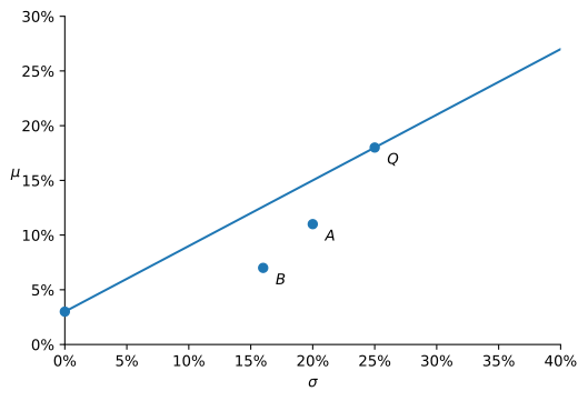
1. In a (\sigma, \mu) diagram, draw the capital allocation line (CAL) of Q, and plot funds A and B. Which portfolios are efficient? Why?
2. Aditya wants to invest in an efficient portfolio (i.e. maximum Sharpe ratio) that offers an expected return of 24%. What should he do? Specify in which assets he should invest, and the standard deviation of such portfolio.
3. Rosalind, on the other hand, for regulatory reasons can only invest in funds A and B (and not the risk-free asset). She is aiming for an expected return of 9%. What would you recommend to her? Please clearly indicate the composition and the standard deviation of such portfolio. Is her portfolio efficient?

Solution.

1. The capital allocation line of Q starts at r_f = 3\% and has slope equal to the Sharpe ratio of Q, S_Q = \frac{0.18 - 0.03}{0.25} = 0.60. The Sharpe ratios of the funds are S_A = \frac{0.11 - 0.03}{0.20} = 0.40, \qquad S_B = \frac{0.07 - 0.03}{0.16} = 0.25, so both lie below the line (Figure 1). The efficient portfolios are those on the capital allocation line of Q: since Q has the highest Sharpe ratio in the economy, no portfolio offers a higher expected return for the same volatility. Funds A and B are inefficient: a mix of Q and the risk-free asset with the same volatility has a higher expected return.

Figure 1: The capital allocation line of Q and funds A and B.

2. Aditya should hold a mix of Q and the risk-free asset on the capital allocation line. The weight y in Q solves 0.03 + y \times (0.18 - 0.03) = 0.24 \quad\Longrightarrow\quad y = \frac{0.21}{0.15} = 1.4. He invests 140% of his wealth in Q, borrowing 40% of his wealth at the risk-free rate. The standard deviation of his portfolio is 1.4 \times 25\% = 35\%.
3. With only A and B, the weight in A that gives 9% solves w_A \times 11\% + (1 - w_A) \times 7\% = 9\% \quad\Longrightarrow\quad w_A = 0.5, so the only portfolio that meets her target is 50% in A and 50% in B. The covariance is 0.25 \times 0.20 \times 0.16 = 0.008, so \sigma^2 = 0.5^2 \times 0.20^2 + 0.5^2 \times 0.16^2 + 2 \times 0.5 \times 0.5 \times 0.008 = 0.0204, and \sigma = 14.28\%. Her portfolio is not efficient: its Sharpe ratio is (0.09 - 0.03)/0.1428 = 0.42, below the 0.60 of Q. On the capital allocation line of Q, a 9% expected return requires a volatility of only (0.09 - 0.03)/0.60 = 10\%. Within A and B alone, though, there is no better choice: it is the only portfolio of the two funds that delivers 9%.

Problem 4 Two risky assets A and B have the following characteristics:

• \operatorname{E}(R_{A}) = 0.10, \sigma_{A} = 0.10
• \operatorname{E}(R_{B}) = 0.15, \sigma_{B} = 0.25
• \rho_{AB} = +1

1. Suppose that you aim for an expected return of 5%, what should be the composition of your portfolio? What is the risk of that portfolio? Explain how this strategy can be possible.
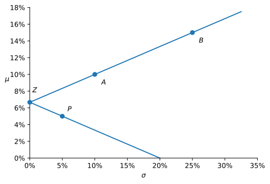
2. Draw the investment opportunity set and clearly identify the minimum variance portfolio. Determine its composition and its characteristics.
3. Suppose that in addition to A and B, there is a risk-free asset offering a return of 4%. Is there an arbitrage opportunity? If so, clearly explain how an investor could arbitrage this opportunity (what he buys and what he sells).

Solution.

1. The weight in A that gives 5% solves w_A \times 10\% + (1 - w_A) \times 15\% = 5\% \quad\Longrightarrow\quad w_A = 2, \quad w_B = -1. You short B in an amount equal to your wealth and invest twice your wealth in A. With \rho_{AB} = 1, the volatility of the portfolio is \sigma = |w_A \sigma_A + w_B \sigma_B| = |2 \times 0.10 - 1 \times 0.25| = 5\%. The strategy is possible because the return on B is an exact linear function of the return on A: the two assets always move together, so the short position in B offsets most of the risk of the long position in A.
2. The volatility |w_A \sigma_A + (1 - w_A) \sigma_B| is zero when w_A = \frac{\sigma_B}{\sigma_B - \sigma_A} = \frac{0.25}{0.15} = 1.6667, \qquad w_B = -0.6667. The minimum variance portfolio Z is riskless, with expected return \operatorname{E}[R_Z] = 1.6667 \times 10\% - 0.6667 \times 15\% = 6.67\%. The investment opportunity set is made of two straight lines that meet at Z (Figure 2). The upper line goes through A and B and holds the portfolios with w_A < 1.6667; the lower line holds the portfolios with w_A > 1.6667, including the 5% portfolio P of part a.

Figure 2: The investment opportunity set of A and B with \rho_{AB} = 1.

3. Yes. Portfolio Z is riskless and earns 6.67%, while the risk-free asset earns 4%. An investor borrows at 4% and invests the proceeds in Z. For each $1 borrowed, they buy $1.67 of A and short $0.67 of B, which costs exactly $1. One year later the position is worth $1.0667 for sure, the loan costs $1.04, and the investor keeps $0.0267 with no money down and no risk. Scaling up the position scales the profit, so the prices of A, B and the risk-free asset cannot all stay where they are.

Problem 5 Consider an economy spanned by N risky assets and a risk-free asset. The tangency portfolio (Q) has an expected return of 16% and a standard deviation of 20%. You also know that Dmitri chooses to optimally invest in portfolio (P_{1}) with an expected return of 13% and a standard deviation of 14%.

1. Compute the risk-free rate r_{f} of this economy.
2. What is the composition of the portfolio owned by Dmitri?
3. Ingrid wants to invest optimally in a portfolio (P_{2}) that has a standard deviation of 30%. What would you recommend to her? Please clearly indicate the composition of her portfolio, and the expected return that she will be able to achieve.

Solution.

1. Dmitri invests optimally, so P_1 lies on the capital allocation line of Q and has the same Sharpe ratio: \frac{0.16 - r_f}{0.20} = \frac{0.13 - r_f}{0.14} \quad\Longrightarrow\quad 14 (16 - r_f) = 20 (13 - r_f) \quad\Longrightarrow\quad r_f = 6\%.
2. His weight in Q is y = 0.14 / 0.20 = 0.70, so he holds 70% in Q and 30% in the risk-free asset. As a check, 6\% + 0.70 \times (16\% - 6\%) = 13\%.
3. Ingrid should also hold a mix of Q and the risk-free asset, with y = 0.30 / 0.20 = 1.5: 150% of her wealth in Q, financed by borrowing 50% of her wealth at the risk-free rate. Her expected return is \operatorname{E}[r_{P_2}] = 6\% + 1.5 \times (16\% - 6\%) = 21\%.