Poisson Processes

Many events in finance arrive at unpredictable moments: a firm defaults, an insurance claim is filed, an order reaches the exchange, a central bank surprises the market, or a stock price jumps on news. The Poisson process is the basic model for the times at which such events occur. It counts how many events have happened up to each point in time, and it rests on two assumptions: events arrive at a constant average rate, and what happens over one period of time tells us nothing about what will happen over another.

The Poisson process is the first process in continuous time that we study. It arises from the Poisson limit of sums of Bernoulli random variables, its paths are simple to draw, and most calculations require nothing beyond generating functions and martingales. Its continuous counterpart, a process that moves all the time by tiny amounts instead of by jumps, is Brownian motion.

These notes draw on Grimmett and Stirzaker (2001) and on the treatment of jump processes in Shreve (2004).

Grimmett, Geoffrey, and David Stirzaker. 2001. Probability and Random Processes. 3rd ed. Oxford University Press.

Shreve, Steven E. 2004. Stochastic Calculus for Finance II: Continuous-Time Models. Springer Finance. Springer.

Counting Events in Continuous Time

A Bernoulli Construction

Suppose that events can occur at any moment, at an average rate of \lambda events per unit of time. To model this, divide the interval [0, t] into n short slots of length \Delta t = t / n. In each slot, an event occurs with probability \lambda \Delta t and no event occurs with probability 1 - \lambda \Delta t, independently across slots. Let X_{j} be the Bernoulli indicator that an event occurs in slot j. The number of events up to time t is N_{t}^{(n)} = X_{1} + X_{2} + \cdots + X_{n}. This is a binomial random variable with n trials and success probability \lambda t / n, so the expected number of events is \lambda t regardless of n.

As the slots become shorter, the probability of an event in each slot shrinks while the number of slots grows. This is exactly the setting of the Poisson limit in the notes on generating functions. The PGF of N_{t}^{(n)} is G_{N_{t}^{(n)}}(z) = \left(1 + \frac{\lambda t (z - 1)}{n}\right)^{n} \xrightarrow[n \to \infty]{} e^{\lambda t (z - 1)}, so in the limit the number of events up to time t has a Poisson distribution with mean \lambda t.

The construction gives us more than the distribution at a single date. For s < t, the events in (s, t] are determined by the slots in that interval, which are independent of the slots in [0, s]. The number of events in (s, t] is again binomial, and in the limit it is Poisson with mean \lambda (t - s), a quantity that depends only on the length of the interval. These properties survive the limit and define the Poisson process.

Definition

WarningPoisson Process

A stochastic process \{N_{t} \colon t \geq 0\} is called a Poisson process with rate (or intensity) \lambda > 0 if it has the following three properties:

1. N_{0} = 0.

2. For any finite set of times 0 \leq t_{0} < t_{1} < \cdots < t_{n}, the increments N_{t_{1}} - N_{t_{0}}, N_{t_{2}} - N_{t_{1}}, \ldots, N_{t_{n}} - N_{t_{n - 1}} are independent.

3. For any 0 \leq s < t, the increment N_{t} - N_{s} has a Poisson distribution with mean \lambda (t - s).

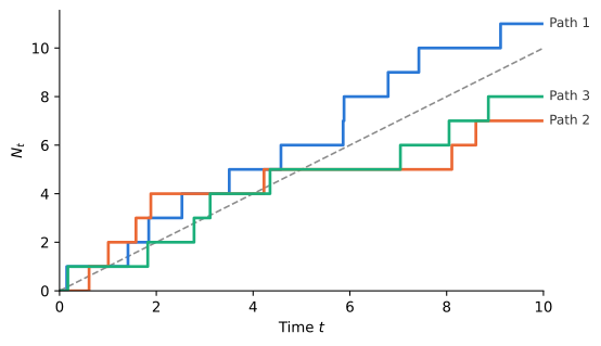
The paths of N_{t} are step functions that start at zero and jump up by one at each event. By convention the paths are right-continuous, so N_{t} includes an event that occurs exactly at time t.

Using the moments of the Poisson distribution, we have \operatorname{E}(N_{t}) = \lambda t, \qquad \operatorname{V}(N_{t}) = \lambda t, \qquad G_{N_{t}}(z) = e^{\lambda t (z - 1)}. The rate \lambda is the expected number of events per unit of time. An insurer whose claims arrive at the rate \lambda = 10 per year, for example, expects ten claims a year.

The Bernoulli construction also describes the behavior of the process over a short interval. Over an interval of length \mathop{}\!\mathrm{d}t, the Poisson probabilities give \begin{aligned} \operatorname{P}(N_{t + \mathop{}\!\mathrm{d}t} - N_{t} = 0) & = e^{-\lambda \mathop{}\!\mathrm{d}t} = 1 - \lambda \mathop{}\!\mathrm{d}t+ o(\mathop{}\!\mathrm{d}t), \\ \operatorname{P}(N_{t + \mathop{}\!\mathrm{d}t} - N_{t} = 1) & = \lambda \mathop{}\!\mathrm{d}t\, e^{-\lambda \mathop{}\!\mathrm{d}t} = \lambda \mathop{}\!\mathrm{d}t+ o(\mathop{}\!\mathrm{d}t), \\ \operatorname{P}(N_{t + \mathop{}\!\mathrm{d}t} - N_{t} \geq 2) & = o(\mathop{}\!\mathrm{d}t), \end{aligned} where o(\mathop{}\!\mathrm{d}t) denotes terms that vanish faster than \mathop{}\!\mathrm{d}t. Over a short interval there is either no event or a single event, and the probability of an event is proportional to the length of the interval. Writing \mathop{}\!\mathrm{d}N_{t} = N_{t + \mathop{}\!\mathrm{d}t} - N_{t}, this says that \mathop{}\!\mathrm{d}N_{t} is approximately a Bernoulli random variable with \operatorname{E}(\mathop{}\!\mathrm{d}N_{t}) = \lambda \mathop{}\!\mathrm{d}t.

Figure 1: The figure plots three simulated paths of a Poisson process with rate \lambda = 1 over 0 \leq t \leq 10. The dashed line denotes \operatorname{E}(N_{t}) = \lambda t.

Combining and Splitting Poisson Processes

Two operations on Poisson processes appear constantly in applications: merging several independent streams of events into one, and splitting one stream into several types. Both follow from the generating function results for Poisson sums and thinning.

WarningSuperposition and Thinning

1. Superposition. If N_{t}^{(1)} and N_{t}^{(2)} are independent Poisson processes with rates \lambda_{1} and \lambda_{2}, then N_{t} = N_{t}^{(1)} + N_{t}^{(2)} is a Poisson process with rate \lambda_{1} + \lambda_{2}.

2. Thinning. If each event of a Poisson process with rate \lambda is independently classified as type A with probability p and as type B with probability 1 - p, then the counts N_{t}^{A} and N_{t}^{B} of each type are independent Poisson processes with rates \lambda p and \lambda (1 - p).

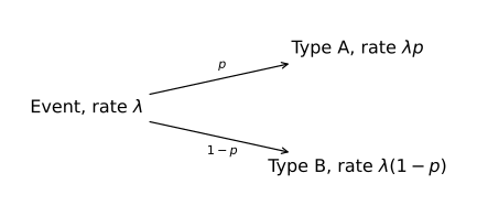
Figure 2 shows the classification behind thinning. Each event of the original process takes one of two branches, independently of the other events and of the times at which they arrive.

Figure 2: The figure shows how thinning classifies each event. An event of the process with rate \lambda is of type A with probability p and of type B with probability 1 - p, which gives two processes with rates \lambda p and \lambda (1 - p).

Proof

For superposition, the sum of independent processes with independent increments has independent increments, and by the notes on generating functions the increment over (s, t] is Poisson with mean (\lambda_{1} + \lambda_{2})(t - s).

For thinning, it is enough to consider a single interval [0, t], since increments over disjoint intervals are built from disjoint sets of events. We compute the joint PGF of N_{t}^{A} and N_{t}^{B} by conditioning on N_{t}. Given N_{t} = n, each of the n events contributes a factor z_{1} if it is of type A and z_{2} if it is of type B, so \operatorname{E}\left(z_{1}^{N_{t}^{A}} z_{2}^{N_{t}^{B}} \mid N_{t} = n\right) = (p z_{1} + (1 - p) z_{2})^{n}. Taking expectations over N_{t} and using its PGF, \operatorname{E}\left(z_{1}^{N_{t}^{A}} z_{2}^{N_{t}^{B}}\right) = e^{\lambda t (p z_{1} + (1 - p) z_{2} - 1)} = e^{\lambda p t (z_{1} - 1)} \, e^{\lambda (1 - p) t (z_{2} - 1)}. The joint PGF factors into the PGF of a \text{Poisson}(\lambda p t) random variable in z_{1} times the PGF of a \text{Poisson}(\lambda (1 - p) t) random variable in z_{2}. Since a joint PGF determines the joint distribution, the two counts are independent Poisson random variables.

The independence of the thinned processes is surprising at first. If we learn that many type A events occurred, we might expect fewer type B events. That intuition is correct when the total number of events is fixed, but here the total is random. Many type A events suggest that the total was large, which exactly offsets the smaller share left for type B. A practice problem in the notes on generating functions works through the same calculation for buy and sell orders arriving at a market maker, and compares it with a fixed number of orders.

Example 1 Suppose large news announcements about a stock arrive as a Poisson process with rate \lambda = 6 per year, and each announcement is good news with probability p = 0.4 and bad news otherwise. Good-news jumps then arrive at rate 2.4 per year and bad-news jumps at rate 3.6 per year, and the two processes are independent. The probability of a year with no bad-news jumps is e^{-3.6} = 0.0273, whatever the number of good-news jumps.

Waiting Times

The First Event

Let T_{1} be the time of the first event. The first event occurs after time t if and only if no event occurs in [0, t], so \operatorname{P}(T_{1} > t) = \operatorname{P}(N_{t} = 0) = e^{-\lambda t}. Therefore, T_{1} has an exponential distribution with rate \lambda, and the expected waiting time for the first event is 1 / \lambda. A firm that defaults at the first event of a Poisson process with intensity \lambda = 0.02 per year waits on average 1 / 0.02 = 50 years for its default.

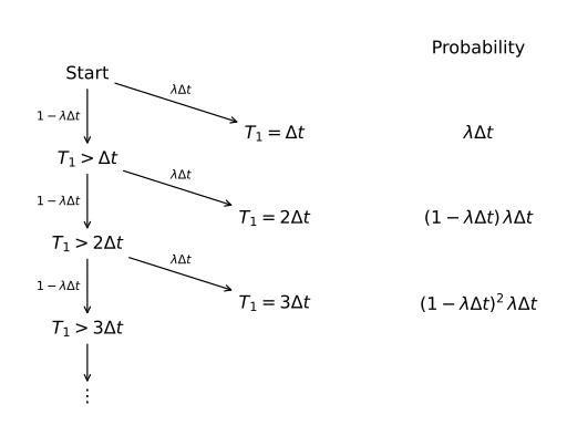
The Bernoulli construction gives the same answer from a different angle. Each slot either holds the first event, with probability \lambda \Delta t, or passes without one, as in Figure 3. The number of slots until the first event is therefore geometric with success probability \lambda \Delta t, and the probability that no event occurs in the first t / \Delta t slots, the probability of reaching row t / \Delta t of the left column, is (1 - \lambda \Delta t)^{t / \Delta t} \xrightarrow[\Delta t \to 0]{} e^{-\lambda t}. The exponential distribution is the continuous-time limit of the geometric distribution, in the same way that the Poisson distribution is the limit of the binomial.

Figure 3: The figure shows the first event in the Bernoulli construction. In each slot of length \Delta t, the first event occurs with probability \lambda \Delta t, and with probability 1 - \lambda \Delta t the process moves down the left column to the next slot. The right column gives the probability that the first event falls in each slot.

Memorylessness

The exponential distribution has a property that makes it the natural model for waiting times in the Poisson process. If T \sim \text{Exp}(\lambda), then for all s, t \geq 0 \operatorname{P}(T > s + t \mid T > s) = \frac{\operatorname{P}(T > s + t)}{\operatorname{P}(T > s)} = \frac{e^{-\lambda (s + t)}}{e^{-\lambda s}} = e^{-\lambda t} = \operatorname{P}(T > t). Having waited s units of time without an event does not change the distribution of the remaining waiting time. This memoryless property characterizes the exponential distribution among continuous distributions on [0, \infty), just as the geometric distribution is the only memoryless distribution on \{1, 2, \ldots\}.

In credit risk, memorylessness means that the probability that a firm defaults over the next year does not depend on how long the firm has survived. The probability of default over a short interval, given survival up to time t, is \operatorname{P}(T \leq t + \mathop{}\!\mathrm{d}t\mid T > t) = 1 - e^{-\lambda \mathop{}\!\mathrm{d}t} = \lambda \mathop{}\!\mathrm{d}t+ o(\mathop{}\!\mathrm{d}t), which is why \lambda is also called the hazard rate of default. Models used in practice let the hazard rate vary over time and with the state of the economy, but the constant-intensity case is the building block.

Interarrival Times

Memorylessness is what lets the process start afresh after each event. Because increments are independent and stationary, once an event has occurred the past carries no information about the future, and the time until the next event is again exponential with rate \lambda, independent of everything that happened before. We state the result without a formal proof.

WarningInterarrival Times

Let T_{1}, T_{2}, \ldots denote the times between consecutive events of a Poisson process with rate \lambda. Then T_{1}, T_{2}, \ldots are independent random variables, each with an \text{Exp}(\lambda) distribution. Conversely, if T_{1}, T_{2}, \ldots are iid \text{Exp}(\lambda) and W_{n} = T_{1} + \cdots + T_{n}, then N_{t} = \max\{n \geq 0 \colon W_{n} \leq t\} is a Poisson process with rate \lambda.

The converse gives a simple recipe to simulate a Poisson process: draw exponential waiting times and add them up. The paths in Figure 1 were generated in this way.

Arrival Times

The time of the n-th event is W_{n} = T_{1} + \cdots + T_{n}, a sum of n independent exponential random variables. By the results in the notes on generating functions, W_{n} has a gamma distribution with M_{W_{n}}(\theta) = \left(\frac{\lambda}{\lambda - \theta}\right)^{n}, \qquad \operatorname{E}(W_{n}) = \frac{n}{\lambda}, \qquad \operatorname{V}(W_{n}) = \frac{n}{\lambda^{2}}. The arrival times and the counts are two descriptions of the same process. The n-th event has occurred by time t if and only if at least n events have occurred in [0, t], so \operatorname{P}(W_{n} \leq t) = \operatorname{P}(N_{t} \geq n) = 1 - \sum_{k = 0}^{n - 1} e^{-\lambda t} \frac{(\lambda t)^{k}}{k!}.

Example 2 A portfolio contains bonds issued by 50 firms, each defaulting at the first event of an independent Poisson process with intensity 0.02 per year. Until the first default occurs, defaults in the portfolio arrive as a Poisson process with rate 50 \times 0.02 = 1 per year, by superposition. Ignoring the small reduction in the rate after each default, the probability that at least two firms default within a year is \operatorname{P}(W_{2} \leq 1) = 1 - e^{-1} (1 + 1) = 1 - 2 e^{-1} = 0.2642.

Martingales of the Poisson Process

Let \mathcal{F}_{t} denote the information generated by observing the process \{N_{s} \colon s \leq t\} up to time t. The definition of a martingale carries over from discrete time: a process \{M_{t}\} adapted to \{\mathcal{F}_{t}\} is a martingale if \operatorname{E}(M_{t} \mid \mathcal{F}_{s}) = M_{s} for all s \leq t. Since increments of the Poisson process are independent of the past, conditional expectations of functions of N_{t} - N_{s} given \mathcal{F}_{s} reduce to ordinary expectations, exactly as for the random walk.

The Poisson process itself is not a martingale, since it only moves up. Its expected increase over (s, t] is \lambda (t - s), and subtracting it produces a martingale.

WarningMartingales of the Poisson Process

Let \{N_{t}\} be a Poisson process with rate \lambda. The following processes are martingales with respect to \{\mathcal{F}_{t}\}:

1. The compensated Poisson process M_{t} = N_{t} - \lambda t.

2. The process M_{t}^{2} - \lambda t.

3. For any real \theta, the exponential martingale Z_{t} = \exp\left(\theta N_{t} - \lambda t (e^{\theta} - 1)\right).

Proof

Fix s < t and write \Delta N = N_{t} - N_{s}, which is independent of \mathcal{F}_{s} and has a Poisson distribution with mean \lambda (t - s). Let \Delta M = M_{t} - M_{s} = \Delta N - \lambda (t - s), so that \operatorname{E}(\Delta M) = 0 and \operatorname{E}(\Delta M^{2}) = \operatorname{V}(\Delta N) = \lambda (t - s).

For the first process, \operatorname{E}(M_{t} \mid \mathcal{F}_{s}) = M_{s} + \operatorname{E}(\Delta M) = M_{s}. For the second, expanding M_{t}^{2} = M_{s}^{2} + 2 M_{s} \Delta M + \Delta M^{2} gives \operatorname{E}(M_{t}^{2} - \lambda t \mid \mathcal{F}_{s}) = M_{s}^{2} + 2 M_{s} \operatorname{E}(\Delta M) + \operatorname{E}(\Delta M^{2}) - \lambda t = M_{s}^{2} + \lambda (t - s) - \lambda t = M_{s}^{2} - \lambda s. For the third, the MGF of a Poisson random variable with mean \lambda (t - s) is \operatorname{E}(e^{\theta \Delta N}) = e^{\lambda (t - s) (e^{\theta} - 1)}, so that \operatorname{E}(Z_{t} \mid \mathcal{F}_{s}) = Z_{s} \, \operatorname{E}\left(e^{\theta \Delta N}\right) e^{-\lambda (t - s) (e^{\theta} - 1)} = Z_{s}.

These three martingales are the continuous-time counterparts of the examples in the notes on discrete-time martingales. The compensated process plays the role of the random walk S_{n}, the second martingale plays the role of S_{n}^{2} - n, and the exponential martingale has the form e^{\theta N_{t} - t K(\theta)}, where K(\theta) = \lambda (e^{\theta} - 1) is the cumulant generating function of N_{1}.

Compound Poisson Processes

In most applications each event carries a size: an insurance claim has an amount, a default causes a loss, and a price jump has a magnitude. Let Y_{1}, Y_{2}, \ldots be iid random variables, independent of the Poisson process \{N_{t}\}, and define X_{t} = \sum_{i = 1}^{N_{t}} Y_{i}, with X_{t} = 0 when N_{t} = 0. The process \{X_{t}\} is called a compound Poisson process. Its paths are step functions, like those of N_{t}, but the jumps have random sizes Y_{i}, which can be positive or negative. A compound Poisson process also has independent and stationary increments.

For each t, X_{t} is a random sum. The argument used in the notes on generating functions for the PGF of a random sum applies to the characteristic function without change: given N_{t} = n, the characteristic function of X_{t} is \phi_{Y}(u)^{n}, so that \phi_{X_{t}}(u) = \operatorname{E}(\phi_{Y}(u)^{N_{t}}) = G_{N_{t}}(\phi_{Y}(u)).

WarningCharacteristic Function of a Compound Poisson Process

If \{X_{t}\} is a compound Poisson process with rate \lambda and jump sizes with characteristic function \phi_{Y}, then \phi_{X_{t}}(u) = e^{\lambda t (\phi_{Y}(u) - 1)}. \tag{1} If \operatorname{E}(Y^{2}) < \infty, then \operatorname{E}(X_{t}) = \lambda t \operatorname{E}(Y) and \operatorname{V}(X_{t}) = \lambda t \operatorname{E}(Y^{2}). When the MGF of Y exists, M_{X_{t}}(\theta) = e^{\lambda t (M_{Y}(\theta) - 1)}.

Proof

The characteristic function follows from G_{N_{t}}(z) = e^{\lambda t (z - 1)} evaluated at z = \phi_{Y}(u). For the moments, write \kappa(u) = \lambda t (\phi_{Y}(u) - 1), so that \phi_{X_{t}} = e^{\kappa}. Differentiating, \phi_{X_{t}}' = \kappa' e^{\kappa} and \phi_{X_{t}}'' = (\kappa'' + \kappa'^{2}) e^{\kappa}. At u = 0 we have \kappa(0) = 0, \kappa'(0) = \lambda t \, i \operatorname{E}(Y), and \kappa''(0) = -\lambda t \operatorname{E}(Y^{2}). Therefore \begin{aligned} \operatorname{E}(X_{t}) & = -i \phi_{X_{t}}'(0) = \lambda t \operatorname{E}(Y), \\ \operatorname{E}(X_{t}^{2}) & = -\phi_{X_{t}}''(0) = \lambda t \operatorname{E}(Y^{2}) + (\lambda t \operatorname{E}(Y))^{2}, \end{aligned} and the variance is \operatorname{E}(X_{t}^{2}) - \operatorname{E}(X_{t})^{2} = \lambda t \operatorname{E}(Y^{2}).

The variance depends on \operatorname{E}(Y^{2}), not on \operatorname{V}(Y), because the randomness of X_{t} comes from two sources: the number of jumps and their sizes. Equation (1) is the reason characteristic functions are the natural tool for jump processes. The density of X_{t} is an infinite mixture over the number of jumps and is rarely available in closed form, whereas its characteristic function is a single exponential. The best-known financial example is the jump-diffusion model of Merton (1976), in which the log price of a stock is the sum of a Brownian component and a compound Poisson process with normally distributed jumps.

Merton, Robert C. 1976. “Option Pricing When Underlying Stock Returns Are Discontinuous.” Journal of Financial Economics 3 (1–2): 125–44.

Example 3 In the Merton model the jumps Y_{i} of the log price are normally distributed with mean m and variance s^{2}. Leaving the Brownian part aside, the characteristic function of the jump component over [0, t] is \phi_{X_{t}}(u) = \exp\left(\lambda t \left(e^{i u m - \frac{1}{2} u^{2} s^{2}} - 1\right)\right). Since the Brownian and jump components are independent, the characteristic function of the log price is the product of this expression and the normal characteristic function of the Brownian part. We return to this model in the notes on pricing with jumps.

Application: Default and Credit Spreads

A simple model of credit risk assumes that a firm defaults at the first event of a Poisson process whose intensity \lambda is the hazard rate of default, as in the section on memorylessness. The default time \tau is then exponential with rate \lambda, and the probability that the firm survives until time T is \operatorname{P}(\tau > T) = e^{-\lambda T}. Consider a zero-coupon bond issued by the firm that pays one dollar at time T if the firm has not defaulted and nothing otherwise. If the risk-free rate is a constant r and bondholders value the bond at its expected payoff discounted at the risk-free rate, the price of the bond is P^{d}(T) = e^{-r T} \operatorname{P}(\tau > T) = e^{-(r + \lambda) T}. The bond is priced as if it were a risk-free bond discounted at the higher rate r + \lambda. Its yield exceeds the risk-free rate by exactly \lambda, so in this model the credit spread equals the default intensity.

Discounting expected payoffs at the risk-free rate ignores any compensation investors require for bearing default risk. The notes on pricing with jumps show that the formula remains valid once expectations are computed under the risk-neutral measure, where \lambda becomes a risk-neutral intensity that is typically larger than the historical default rate. Duffie and Singleton (1999) develop this approach in detail, including random intensities and partial recovery.

Duffie, Darrell, and Kenneth J. Singleton. 1999. “Modeling Term Structures of Defaultable Bonds.” Review of Financial Studies 12 (4): 687–720.

Example 4 A firm has a default intensity of \lambda = 0.02 per year and the risk-free rate is r = 0.04. The probability that the firm survives the next T = 5 years is e^{-0.02 \times 5} = 0.9048. A 5-year zero-coupon bond issued by the firm is worth P^{d}(5) = e^{-(0.04 + 0.02) \times 5} = 0.7408, compared with e^{-0.04 \times 5} = 0.8187 for a risk-free zero-coupon bond with the same maturity. The yield on the defaultable bond is 6%, a credit spread of 200 basis points.

Application: The Insurance Ruin Problem

The classic model of ruin in insurance is due to Lundberg and Cramér. An insurance company starts with capital u > 0 and collects premiums at a constant rate c per unit of time. Claims arrive as a Poisson process with rate \lambda, and the claim sizes Y_{1}, Y_{2}, \ldots are iid, positive, and independent of the arrival times. The surplus of the company at time t is U_{t} = u + c t - X_{t}, \qquad X_{t} = \sum_{i = 1}^{N_{t}} Y_{i}. The company is ruined at the first time \tau its surplus becomes negative, and the ruin probability is \psi(u) = \operatorname{P}(\tau < \infty). On average the surplus grows at the rate c - \lambda \operatorname{E}(Y), which we assume is positive. Otherwise, ruin is certain.

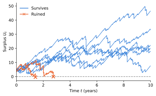
As Figure 4 shows, the surplus rises steadily between claims and falls only when a claim arrives. Ruin therefore happens at a claim larger than the remaining surplus, and the surplus lands below zero by the difference. How far below zero it lands will matter for the ruin probability.

Figure 4: The figure plots eight simulated surplus paths over ten years for an insurer that starts with u = 5, receives \lambda = 10 claims per year with mean 1, and collects premiums at the rate c = 12. Paths that fall below zero are ruined and stop at the ruin time, marked with a cross.

Whether a path is ever ruined depends on its whole future, so \psi(u) cannot be read off the distribution of U_{t} at any single date. As for the gambler in the notes on discrete-time martingales, we use a martingale and compare its value at the start with its value at ruin.

An Exponential Martingale

For the biased gambler in the notes on discrete-time martingales, the martingale was (q / p)^{S_{n}}, a constant raised to the power of the gambler’s wealth. We look for a martingale of the same kind, Z_{t} = e^{-R U_{t}} for some R > 0, with e^{-R} in the role of q / p. Using the MGF of the compound Poisson process, \operatorname{E}(Z_{t}) = Z_{0} \, e^{-c R t} \, \operatorname{E}\left(e^{R X_{t}}\right) = Z_{0} \exp\left(t \left(\lambda (M_{Y}(R) - 1) - c R\right)\right). Premiums pull the exponent down at the rate c R, and claims push it up at the rate \lambda (M_{Y}(R) - 1). The expectation stays at Z_{0} when the two cancel, \lambda (M_{Y}(R) - 1) = c R, \tag{2} and Z is then a martingale, because the increments of X are independent of the past. A positive solution R is called the adjustment coefficient. Both sides of (2) are zero at R = 0, and the left side is convex with initial slope \lambda \operatorname{E}(Y) < c, so it starts below the line c R. It crosses the line at some R > 0 when M_{Y}(\theta) grows without bound as \theta approaches the end of the interval where it is finite: infinity for bounded claims, and the rate parameter for exponential or gamma claims. Heavy-tailed claims, such as Pareto losses from natural catastrophes, have an infinite MGF for every \theta > 0 and no adjustment coefficient.

Stopping at Ruin

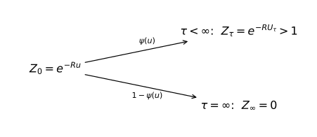
The martingale starts at Z_{0} = e^{-R u}. On a path that is never ruined, the surplus grows without bound and Z_{t} goes to zero. On a path that is ruined, the surplus at ruin is negative and Z_{\tau} = e^{-R U_{\tau}} is larger than one. The martingale keeps its expectation, so e^{-R u} = (1 - \psi(u)) \times 0 + \psi(u) \, \operatorname{E}\left(Z_{\tau} \mid \tau < \infty\right). Figure 5 draws this calculation as a tree with two branches, like the binomial trees that price options. The value today is the probability-weighted average of the values on the two branches, and the ruin probability is the weight on the branch where the company is ruined.

Figure 5: The figure shows the martingale Z_{t} = e^{-R U_{t}} stopped at ruin. With probability \psi(u) the company is ruined and Z_{\tau} is larger than one; with probability 1 - \psi(u) it is never ruined and Z_{t} goes to zero.

WarningRuin Probability

If R > 0 solves (2), then for every initial capital u > 0, \psi(u) = \frac{e^{-R u}}{\operatorname{E}\left(e^{-R U_{\tau}} \mid \tau < \infty\right)} \leq e^{-R u}. \tag{3} The bound is called Lundberg’s inequality.

Proof

The argument above stops the martingale at a time that may be infinite, which needs care: in the notes on discrete-time martingales, a gambler on a fair coin with no upper barrier is ruined with certainty, yet the walk stopped at ruin does not keep its expectation. The proof follows the argument given there for a biased coin. The stopped process Z_{t \land \tau} is a martingale, a result that carries over to continuous time, so for any t e^{-R u} = \operatorname{E}(Z_{t \land \tau}) = \operatorname{E}(Z_{\tau} \mathbf{1}_{\{\tau \leq t\}}) + \operatorname{E}(Z_{t} \mathbf{1}_{\{\tau > t\}}). Let t \to \infty. On each path, Z_{\tau} \mathbf{1}_{\{\tau \leq t\}} is zero before ruin and Z_{\tau} from ruin on, so it increases with t, and by monotone convergence the first term goes to \operatorname{E}(Z_{\tau} \mathbf{1}_{\{\tau < \infty\}}). For the second term, \frac{U_{t}}{t} = \frac{u}{t} + c - \frac{N_{t}}{t} \cdot \frac{1}{N_{t}} \sum_{i = 1}^{N_{t}} Y_{i} \longrightarrow c - \lambda \operatorname{E}(Y) > 0 almost surely, by the strong law of large numbers applied to the claims and to the interarrival times, whose average 1 / \lambda gives N_{t} / t \to \lambda. Hence U_{t} \to \infty and Z_{t} \mathbf{1}_{\{\tau > t\}} \to 0 almost surely. Before ruin the surplus is nonnegative, so Z_{t} \mathbf{1}_{\{\tau > t\}} \leq 1, and by dominated convergence \operatorname{E}(Z_{t} \mathbf{1}_{\{\tau > t\}}) \to 0. Therefore e^{-R u} = \operatorname{E}(Z_{\tau} \mathbf{1}_{\{\tau < \infty\}}) = \psi(u) \, \operatorname{E}(Z_{\tau} \mid \tau < \infty).

The denominator in (3) depends on how far below zero the surplus falls at ruin. The gambler moves in unit steps and lands exactly at zero, so for the gambler the denominator is one and the formula is exact: for a walk that drifts up, with p > q and no upper barrier, it gives a ruin probability of (q / p)^{u}. The insurer’s surplus jumps past zero by an amount that depends on the claims, but in every case Lundberg’s inequality shows that the ruin probability falls exponentially with the capital.

The Deficit with Exponential Claims

When claims are exponential with mean 1 / \eta, the deficit at ruin can be computed. Let V be the surplus just before the claim that causes ruin, so that U_{\tau} = V - Y_{k} when ruin happens at the k-th claim. Whether the company survives the first k - 1 claims, and the surplus v it has just before the k-th, depend only on earlier claims and arrival times, so they are independent of Y_{k}. On that event, ruin at the k-th claim means Y_{k} > v. For y \geq 0, \operatorname{P}(U_{\tau} < -y \mid \text{ruin at claim } k, V = v) = \operatorname{P}(Y_{k} > v + y \mid Y_{k} > v) = \operatorname{P}(Y_{k} > y) = e^{-\eta y}, where the second step is the memoryless property of the exponential distribution. The answer depends neither on k nor on v, so averaging over both by the law of total probability gives \operatorname{P}(U_{\tau} < -y \mid \tau < \infty) = e^{-\eta y}. Given ruin, the deficit -U_{\tau} has the same distribution as a claim, however close to zero the company was.

Example 5 With exponential claims, M_{Y}(\theta) = \eta / (\eta - \theta) for \theta < \eta, and (2) becomes \lambda R / (\eta - R) = c R, with positive solution R = \eta - \lambda / c. Given ruin, U_{\tau} \sim -Y, and \operatorname{E}\left(e^{-R U_{\tau}} \mid \tau < \infty\right) = \operatorname{E}\left(e^{R Y}\right) = \frac{\eta}{\eta - R} = \frac{c \eta}{\lambda}. Substituting into (3), \psi(u) = \frac{\lambda}{c \eta} e^{-(\eta - \lambda / c) u}. The ruin probability falls with the capital u, which enters only through the exponential decay. It also falls with the premium rate c and rises with the claim rate \lambda and the mean claim 1 / \eta, each of which moves the factor and the decay rate in the same direction.

The insurer in Figure 4 receives \lambda = 10 claims per year with a mean size of 1 million dollars and collects premiums of c = 12 million dollars per year, 20% above expected claims. The adjustment coefficient is R = 1 - 10 / 12 = 1/6. With an initial capital of u = 5 million dollars, Lundberg’s bound is e^{-5/6} = 0.4346 and the exact ruin probability is \frac{10}{12} e^{-5/6} = 0.3622. A simulation of 4000 surplus paths over about 150 years, long enough that later ruin is negligible, yields a ruin frequency of 0.364. To bring the ruin probability down to 1%, the insurer needs capital of u = 6 \ln(100 \times 10 / 12) = 26.5 million dollars.

Practice Problems

Problem 1 Orders reach a market maker as a Poisson process with rate \lambda = 3 per minute.

1. Compute the probability that no order arrives during a given minute, and the probability that at least two arrive.
2. Compute the mean and standard deviation of the waiting time until the fifth order.
3. Exactly one order arrived during the first minute. What is the probability that exactly four orders have arrived by the end of the second minute?

Solution

1. \operatorname{P}(N_{1} = 0) = e^{-3} = 0.0498 and \operatorname{P}(N_{1} \geq 2) = 1 - e^{-3} (1 + 3) = 1 - 4 e^{-3} = 0.801.
2. The fifth arrival time W_{5} is a sum of five independent \text{Exp}(3) waiting times, so \operatorname{E}(W_{5}) = 5/3 = 1.67 minutes and \operatorname{SD}(W_{5}) = \sqrt{5} / 3 = 0.745 minutes.
3. Four orders by the end of the second minute and one in the first means three in the second. The increment N_{2} - N_{1} is independent of N_{1} and has a \text{Poisson}(3) distribution, so the probability is \operatorname{P}(N_{2} - N_{1} = 3) = e^{-3} \, 3^{3} / 3! = 4.5 \, e^{-3} = 0.224. What happened in the first minute is irrelevant.

Problem 2 A firm defaults at the first event of a Poisson process with intensity \lambda = 0.03 per year.

1. Compute the probability that the firm defaults within five years.
2. The firm has survived for ten years. Compute the probability that it defaults within the next five years.
3. Compute the median and the mean of the default time, and the probability that the firm survives beyond the mean. Why is the median below the mean?

Solution

1. \operatorname{P}(\tau \leq 5) = 1 - e^{-0.03 \times 5} = 1 - e^{-0.15} = 0.139.
2. By memorylessness, \operatorname{P}(\tau \leq 15 \mid \tau > 10) = \operatorname{P}(\tau \leq 5) = 0.139. Surviving ten years does not make the firm safer or riskier in this model.
3. The median solves e^{-0.03 m} = 1/2, so m = \ln 2 / 0.03 = 23.1 years, while the mean is 1 / 0.03 = 33.3 years. The probability of surviving beyond the mean is e^{-1} = 0.368. The exponential distribution is skewed to the right: most firms default well before the mean, and a few survive for a very long time and pull the mean up.

Problem 3 (★) Three firms default at independent exponential times \tau_{1}, \tau_{2}, \tau_{3} with intensities \lambda_{1} = 0.01, \lambda_{2} = 0.02, and \lambda_{3} = 0.03 per year.

1. Show that the first default time \min(\tau_{1}, \tau_{2}, \tau_{3}) is exponential with rate \lambda_{1} + \lambda_{2} + \lambda_{3}, and compute its mean.
2. Show that \operatorname{P}(\tau_{3} < \min(\tau_{1}, \tau_{2})) = \lambda_{3} / (\lambda_{1} + \lambda_{2} + \lambda_{3}). Hint: condition on \tau_{3}.
3. A first-to-default bond pays one dollar in five years if none of the three firms has defaulted. With a risk-free rate of 4%, price it as in the notes, and compare it with a five-year bond of the riskiest firm alone.

Solution

1. The first default comes after t only if each firm survives to t, so by independence \operatorname{P}(\min_{i} \tau_{i} > t) = e^{-\lambda_{1} t} e^{-\lambda_{2} t} e^{-\lambda_{3} t} = e^{-(\lambda_{1} + \lambda_{2} + \lambda_{3}) t}. The rate is 0.06 and the mean is 1 / 0.06 = 16.7 years.
2. Write \lambda = \lambda_{1} + \lambda_{2} + \lambda_{3}. Given \tau_{3} = t, firm 3 defaults first if the other two survive to t, which by the first part has probability e^{-(\lambda_{1} + \lambda_{2}) t}. Averaging over the density of \tau_{3}, \operatorname{P}(\tau_{3} < \min(\tau_{1}, \tau_{2})) = \int_{0}^{\infty} \lambda_{3} e^{-\lambda_{3} t} e^{-(\lambda_{1} + \lambda_{2}) t} \mathop{}\!\mathrm{d}t= \frac{\lambda_{3}}{\lambda}, which is 0.03 / 0.06 = 1/2. Each firm is first with probability proportional to its intensity, as thinning suggests: the merged stream of defaults has rate \lambda, and each event belongs to firm i with probability \lambda_{i} / \lambda.
3. The bond pays if the first default occurs after five years, so its price is e^{-(0.04 + 0.06) \times 5} = e^{-0.5} = 0.607, with a spread equal to the sum of the three intensities. A bond of firm 3 alone is worth e^{-(0.04 + 0.03) \times 5} = 0.705. The first-to-default bond is exposed to every firm in the basket.

Problem 4 (★) Let \{N_{t}\} be a Poisson process with rate \lambda, and let 0 < s < t.

1. Show that, given N_{t} = n, N_{s} has the binomial distribution with n trials and success probability s / t. Hint: write N_{t} = N_{s} + (N_{t} - N_{s}).
2. Conclude that, given N_{t} = 1, the time of the event is uniformly distributed on [0, t].
3. A loan book had four defaults last year. Compute the probability that all four occurred in the first half of the year, and the expected number in the first quarter. Does the answer depend on \lambda?

Solution

1. For 0 \leq k \leq n, independence of increments gives \operatorname{P}(N_{s} = k \mid N_{t} = n) = \frac{\operatorname{P}(N_{s} = k) \operatorname{P}(N_{t} - N_{s} = n - k)}{\operatorname{P}(N_{t} = n)} = \frac{e^{-\lambda s} \frac{(\lambda s)^{k}}{k!} \, e^{-\lambda (t - s)} \frac{(\lambda (t - s))^{n - k}}{(n - k)!}}{e^{-\lambda t} \frac{(\lambda t)^{n}}{n!}} = \binom{n}{k} \left(\frac{s}{t}\right)^{k} \left(1 - \frac{s}{t}\right)^{n - k}.
2. With n = 1, \operatorname{P}(T_{1} \leq s \mid N_{t} = 1) = \operatorname{P}(N_{s} = 1 \mid N_{t} = 1) = s / t, the CDF of the uniform distribution on [0, t]. Each event is equally likely to have occurred at any moment of the interval.
3. With n = 4 and s / t = 1/2, the probability is (1/2)^{4} = 0.0625, and the expected number in the first quarter is 4 \times 1/4 = 1. Neither depends on \lambda: once we know how many events occurred, they are spread over the interval like independent uniform draws.

Problem 5 (★) Leave the Brownian part of the Merton model aside, so the log price over one year is X_{1} = \sum_{i = 1}^{N_{1}} Y_{i}, with \lambda = 2 jumps per year and jumps Y_{i} \sim \mathcal{N}(m, s^{2}), where m = -0.05 and s = 0.10.

1. Compute \operatorname{E}(X_{1}), \operatorname{SD}(X_{1}), and the probability that the log price does not move during the year.
2. Rederive \operatorname{V}(X_{t}) = \lambda t \operatorname{E}(Y^{2}) from \operatorname{V}(X_{t}) = \operatorname{E}(\operatorname{V}(X_{t} \mid N_{t})) + \operatorname{V}(\operatorname{E}(X_{t} \mid N_{t})).
3. Show that the cumulant generating function of X_{t} is \lambda t (M_{Y}(\theta) - 1), so that its k-th cumulant is \lambda t \operatorname{E}(Y^{k}). Compute the skewness of X_{1}.

Solution

1. \operatorname{E}(X_{1}) = \lambda m = -0.10 and \operatorname{V}(X_{1}) = \lambda (m^{2} + s^{2}) = 2 (0.0025 + 0.01) = 0.025, so \operatorname{SD}(X_{1}) = 0.158. The log price stays put if no jump occurs, with probability e^{-2} = 0.135, so the distribution of X_{1} has an atom at zero.
2. Given N_{t}, X_{t} is a sum of N_{t} independent jumps, so \operatorname{E}(X_{t} \mid N_{t}) = N_{t} \operatorname{E}(Y) and \operatorname{V}(X_{t} \mid N_{t}) = N_{t} \operatorname{V}(Y). Therefore \operatorname{V}(X_{t}) = \lambda t \operatorname{V}(Y) + \lambda t \operatorname{E}(Y)^{2} = \lambda t \operatorname{E}(Y^{2}), using \operatorname{E}(N_{t}) = \operatorname{V}(N_{t}) = \lambda t.
3. K_{X_{t}}(\theta) = \ln M_{X_{t}}(\theta) = \lambda t (M_{Y}(\theta) - 1), and the k-th derivative at zero is \lambda t M_{Y}^{(k)}(0) = \lambda t \operatorname{E}(Y^{k}). For a normal jump, \operatorname{E}(Y^{3}) = m^{3} + 3 m s^{2} = -0.000125 - 0.0015 = -0.001625, so the third cumulant is 2 \times (-0.001625) = -0.00325 and the skewness is -0.00325 / 0.025^{3/2} = -0.82. Jumps that are negative on average make the distribution of returns skewed to the left, a feature of stock returns that a normal model cannot produce.

Problem 6 (★) Let W_{n} be the time of the n-th event of a Poisson process with rate \lambda, and let r > 0 be the interest rate.

1. Use the MGF of W_{n} to show that the present value of one dollar paid at time W_{n} is \operatorname{E}(e^{-r W_{n}}) = \left(\lambda / (\lambda + r)\right)^{n}.
2. A reinsurer must pay $1 million at the third major hurricane. Hurricanes arrive at rate \lambda = 0.1 per year and r = 0.04. Compute the present value of the obligation.
3. A perpetual bond pays a coupon at the rate of $5 per year until the issuer defaults at the first event of a Poisson process with intensity \lambda = 0.02, and nothing afterwards. Show that its value is c / (r + \lambda), where c is the coupon rate, and compute it for r = 0.04. Compare with the risk-free perpetuity.

Solution

1. \operatorname{E}(e^{-r W_{n}}) = M_{W_{n}}(-r) = \left(\frac{\lambda}{\lambda - (-r)}\right)^{n} = \left(\frac{\lambda}{\lambda + r}\right)^{n}. Each waiting time contributes an independent discount factor \operatorname{E}(e^{-r T_{i}}) = \lambda / (\lambda + r).
2. (0.1 / 0.14)^{3} = 0.364, so the obligation is worth $364,000 today.
3. The coupon paid over [t, t + \mathop{}\!\mathrm{d}t] is c \mathop{}\!\mathrm{d}t if the issuer has survived to t, which happens with probability e^{-\lambda t}. Discounting and adding up, \int_{0}^{\infty} c \, e^{-r t} e^{-\lambda t} \mathop{}\!\mathrm{d}t= \frac{c}{r + \lambda} = \frac{5}{0.06} = 83.3, compared with 5 / 0.04 = 125 for the risk-free perpetuity. As for the zero-coupon bond in the notes, default risk acts like a higher discount rate r + \lambda.

Problem 7 (★★) A stock price moves by one tick at the events of a Poisson process with rate \lambda, up or down with probability 1/2 each, independently of the event times. Its change since time zero is the compound Poisson process X_{t} = \sum_{i = 1}^{N_{t}} Y_{i}, with Y_{i} = \pm 1.

1. Use thinning to write X_{t} = N_{t}^{u} - N_{t}^{d} as the difference of two independent Poisson processes, and compute \operatorname{E}(X_{t}) and \operatorname{V}(X_{t}).
2. Show that X_{t} and X_{t}^{2} - \lambda t are martingales, and that \exp\left(\theta X_{t} - \lambda t (\cosh \theta - 1)\right) is a martingale for every \theta.
3. Explain how X_{t} relates to the simple symmetric random walk, and compare the three martingales with those in the notes on discrete-time martingales.

Solution

1. Classify each tick as up or down. By thinning, the numbers of up and down ticks are independent Poisson processes with rate \lambda / 2 each, and X_{t} = N_{t}^{u} - N_{t}^{d}. Therefore \operatorname{E}(X_{t}) = \lambda t / 2 - \lambda t / 2 = 0 and \operatorname{V}(X_{t}) = \lambda t / 2 + \lambda t / 2 = \lambda t, which matches \lambda t \operatorname{E}(Y^{2}).
2. The increment \Delta X = X_{t} - X_{s} is independent of \mathcal{F}_{s}, with mean zero and variance \lambda (t - s). The first two martingales follow exactly as in the proof for the compensated Poisson process. For the third, M_{Y}(\theta) = \frac{1}{2} (e^{\theta} + e^{-\theta}) = \cosh \theta, so \operatorname{E}(e^{\theta \Delta X}) = e^{\lambda (t - s)(\cosh \theta - 1)}, which cancels the change in the compensating term.
3. X_{t} = S_{N_{t}} is a simple symmetric random walk observed at the random number of steps N_{t}: the walk runs on a Poisson clock. The martingales X_{t}, X_{t}^{2} - N_{t}, and \exp(\theta X_{t}) / (\cosh \theta)^{N_{t}} are S_{n}, S_{n}^{2} - n, and e^{\theta S_{n}} / (\cosh \theta)^{n} with n replaced by N_{t}. The second is a martingale because X_{t}^{2} - N_{t} = (X_{t}^{2} - \lambda t) - (N_{t} - \lambda t) is a difference of two martingales, and the last because each tick multiplies it by e^{\theta Y_{i}} / \cosh \theta, a factor with mean one that is independent of the past. The versions with \lambda t replace the random clock by its expectation.

Problem 8 (★★) An insurer receives claims at rate \lambda = 1 per year and collects premiums at the rate c = 1.2 per year, in millions of dollars.

1. Every claim is exactly $1 million. Write the equation for the adjustment coefficient R, solve it numerically, and compute Lundberg’s bound on the ruin probability for an initial capital of u = 10.
2. Claims are instead exponential with mean $1 million. Compute R, the bound, and the exact ruin probability for u = 10.
3. Use e^{x} \geq 1 + x + \frac{1}{2} x^{2} for x \geq 0 to show that for any positive claims R \leq \frac{2 (c - \lambda \operatorname{E}(Y))}{\lambda \operatorname{E}(Y^{2})}. Evaluate the bound in both cases, and explain why two claim distributions with the same mean lead to different capital requirements.

Solution

1. With M_{Y}(R) = e^{R}, (2) becomes e^{R} - 1 = 1.2 R. The function e^{R} - 1 - 1.2 R is negative just above zero and positive for large R, and a few steps of bisection or Newton’s method give R = 0.354. The bound is e^{-10 \times 0.354} = 0.029.
2. From Example 5, R = \eta - \lambda / c = 1 - 1 / 1.2 = 1/6. The bound is e^{-10/6} = 0.189, and the exact ruin probability is \frac{\lambda}{c \eta} e^{-R u} = \frac{1}{1.2} \times 0.189 = 0.157.
3. Since R Y \geq 0, M_{Y}(R) - 1 = \operatorname{E}(e^{R Y} - 1) \geq R \operatorname{E}(Y) + \frac{1}{2} R^{2} \operatorname{E}(Y^{2}). Substituting into (2), c R = \lambda (M_{Y}(R) - 1) \geq \lambda R \operatorname{E}(Y) + \tfrac{1}{2} \lambda R^{2} \operatorname{E}(Y^{2}), and dividing by R > 0 and rearranging gives the bound. Fixed claims have \operatorname{E}(Y^{2}) = 1 and the bound is 0.4, while exponential claims have \operatorname{E}(Y^{2}) = 2 and the bound is 0.2. The premium loading c - \lambda \operatorname{E}(Y) is the same, but more variable claims push the surplus down by larger amounts, so the ruin probability decays more slowly in the capital. With exponential claims, the insurer needs about twice as much capital to reach the same ruin probability.