Martingales in Discrete Time

All the stochastic processes that we will study in this class will be generated from a sequence of random variables. The specific sequence used to generate the stochastic process \{M_{n}: 0 \leq n < \infty\} determines the information set \mathcal{F}_{n} available at time n. As time passes, we learn more about the processes and what was used to generate the process.

We call the collection of information sets \{\mathcal{F}_{n}: 0 \leq n < \infty\} a filtration. Since information accumulates over time, we always have that \mathcal{F}_{m} \subset \mathcal{F}_{n} for m < n.

Martingales

Earlier, we defined the simple random walk as the process \{S_{n}: 0 \leq n < \infty\}, built from a sequence \{X_{n}: 1 \leq n < \infty\} of independent random variables, where S_{n} = S_{0} + \sum_{i = 1}^{n} X_{i} for n \geq 1. Each X_{i} is a fair coin toss, taking values -1 or 1 with probability 1/2. At time n, the outcomes of the first n coin tosses are known, so the information set is \mathcal{F}_{n} = \{X_{1}, X_{2}, \ldots, X_{n}\}, containing all information revealed by X_{1}, X_{2}, \ldots, X_{n}.

We can then see that \operatorname{E}(S_{n + 1} \mid \mathcal{F}_{n}) = \operatorname{E}(S_{n} + X_{n + 1} \mid \mathcal{F}_{n}) = S_{n} + \operatorname{E}(X_{n + 1} \mid \mathcal{F}_{n}). There is an implicit assumption that the coin tosses are independent from each other. Intuitively, we do not expect to gain any information from the first n tosses to determine the next one. Thus, \operatorname{E}(X_{n + 1} \mid \mathcal{F}_{n}) = \operatorname{E}(X_{n + 1}) = 0, implying \operatorname{E}(S_{n + 1} \mid \mathcal{F}_{n}) = S_{n}.

The process just defined is what we call a martingale. A martingale is a stochastic process \{M_{n}\} adapted to a filtration \{\mathcal{F}_{n}\} such that for all n, \operatorname{E}(M_{n+1} \mid \mathcal{F}_{n}) = M_{n}. In other words, given all the information up to time n, the expected value of the next observation is equal to the current value. This property captures the idea that, on average, the process does not “drift” up or down given the available information.

Example 1 We can generalize the simple random walk by defining \{X_{n}: 1 \leq n < \infty\} as a sequence of independent random variables such that \operatorname{E}(X_{n}) = 0 for all n \geq 1. We do not assume any specific distribution nor we assume that the random variables are identically distributed. We can then define S_{n} = S_{0} + \sum_{i = 1}^{n} X_{i}. We can do as before to find \operatorname{E}(S_{n + 1} \mid \mathcal{F}_{n}) = \operatorname{E}(S_{n} + X_{n + 1} \mid \mathcal{F}_{n}) = S_{n} + \operatorname{E}(X_{n + 1} \mid \mathcal{F}_{n}) = S_{n} + \operatorname{E}(X_{n + 1}) = S_{n}, showing that \{S_{n}\} is a martingale with respect to \{\mathcal{F}_{n}\}.

Example 2 Let \{X_{n}: 1 \leq n < \infty\} be a sequence of independent random variables with \operatorname{E}(X_{n}) = 0 and \operatorname{V}(X_{n}) = \sigma^{2} for all n \geq 1. We do not require the random variables to be identically distributed, but each has mean zero and variance \sigma^{2}. Define S_{n} as in Example 1, and set M_{n} = S_{n}^{2} - n \sigma^{2}. Expanding M_{n+1}, M_{n+1} = (S_{n} + X_{n+1})^{2} - (n+1)\sigma^{2} = S_{n}^{2} + 2S_{n}X_{n+1} + X_{n+1}^{2} - (n+1)\sigma^{2}. Taking conditional expectation, \operatorname{E}(M_{n+1} \mid \mathcal{F}_{n}) = S_{n}^{2} + 2S_{n}\operatorname{E}(X_{n+1} \mid \mathcal{F}_{n}) + \operatorname{E}(X_{n+1}^{2} \mid \mathcal{F}_{n}) - (n+1)\sigma^{2}. Because X_{n+1} is independent of \mathcal{F}_{n}, we have \operatorname{E}(X_{n+1} \mid \mathcal{F}_{n}) = 0 and \operatorname{E}(X_{n+1}^{2} \mid \mathcal{F}_{n}) = \sigma^{2}. Therefore, \operatorname{E}(M_{n+1} \mid \mathcal{F}_{n}) = S_{n}^{2} + \sigma^{2} - (n+1)\sigma^{2} = S_{n}^{2} - n\sigma^{2} = M_{n}. Thus, \{M_{n}\} is a martingale with respect to \{\mathcal{F}_{n}\}.

Example 3 Let \{X_{n}: 1 \leq n < \infty\} be a sequence of independent random variables with X_{n} > 0 and \operatorname{E}(X_{n}) = 1 for all n \geq 1. Set M_{0} = 1 and define M_{n} = X_{1} X_{2} \cdots X_{n}. Since M_{n+1} = M_{n} X_{n+1}, we have \operatorname{E}(M_{n+1} \mid \mathcal{F}_{n}) = M_{n} \operatorname{E}(X_{n+1} \mid \mathcal{F}_{n}) = M_{n} \operatorname{E}(X_{n+1}) = M_{n}. Therefore, \{M_{n}\} is a martingale with respect to \{\mathcal{F}_{n}\}.

Betting Strategies

A gambler does not have to bet the same amount on every round. Suppose that M_{k} - M_{k - 1} is the gain from a bet of one dollar on round k, where \{M_{n}\} is a martingale, and that the gambler stakes H_{k} dollars on that round. The stake must be chosen before the round is played, so H_{k} can depend on everything observed up to time k - 1 but not on the outcome of round k. In other words, H_{k} is \mathcal{F}_{k - 1} measurable, and we say that the sequence \{H_{k}\} is predictable. Starting from W_{0}, the wealth of the gambler after n rounds is W_{n} = W_{0} + \sum_{k = 1}^{n} H_{k} (M_{k} - M_{k - 1}). The process \{W_{n}\} is called a martingale transform. In finance, M_{k} is a (discounted) price, H_{k} is the number of shares held from k - 1 to k, and W_{n} is the value of a self-financing trading strategy.

WarningBetting Strategies Cannot Beat a Martingale

If \{M_{n}\} is a martingale with respect to \{\mathcal{F}_{n}\} and \{H_{k}\} is predictable with each H_{k} bounded, then \{W_{n}\} is a martingale with respect to \{\mathcal{F}_{n}\}. In particular, \operatorname{E}(W_{n}) = W_{0} for every n.

Proof.

Since W_{n + 1} = W_{n} + H_{n + 1} (M_{n + 1} - M_{n}) and H_{n + 1} is known at time n, \operatorname{E}(W_{n + 1} \mid \mathcal{F}_{n}) = W_{n} + H_{n + 1} \left(\operatorname{E}(M_{n + 1} \mid \mathcal{F}_{n}) - M_{n}\right) = W_{n}. The bound on H_{n + 1} guarantees that the expectations exist.

No rule for sizing bets based on past outcomes can turn a fair game into a favorable one. The notes on stochastic calculus define the Itô integral as the continuous-time limit of these sums, with the integrand in the role of H_{k} and the increments of Brownian motion in the role of M_{k} - M_{k - 1}, and the result above becomes the martingale property of the Itô integral.

Example 4 The oldest betting system is the one that gave martingales their name. A gambler bets one dollar on a fair coin and doubles the stake after every loss, stopping at the first win. If the first win comes on round k, the gambler has lost 1 + 2 + \cdots + 2^{k - 2} = 2^{k - 1} - 1 dollars and then wins 2^{k - 1}, for a net gain of one dollar. A win eventually comes with probability one, so the strategy seems to guarantee a profit. Over n rounds, however, the gambler wins one dollar with probability 1 - 2^{-n} and loses 2^{n} - 1 dollars with probability 2^{-n}, so \operatorname{E}(W_{n}) = (1 - 2^{-n}) - 2^{-n} (2^{n} - 1) = 0, as the result above requires. The sure profit at the stopping time is paid for by an unbounded line of credit.

Figure 1 shows why the system is tempting. Five gamblers restart it after every win, so each gains one dollar per cycle, about one dollar every two rounds. Most of the time their wealth climbs steadily, but a run of k losses costs 2^{k} - 1 dollars before the next win recovers it, and at one point a gambler is down 461 dollars. The repeated system is still a betting strategy with stakes that are bounded at each round, so \operatorname{E}(W_{n}) = 0 for every n. At any given round, the few gamblers in the middle of a long losing streak are down by enough to offset the steady gains of all the others.

Figure 1: The figure plots the wealth of five gamblers who use the doubling strategy on a fair coin and restart it after every win. Each downward spike is a losing streak, which the next win recovers in full.

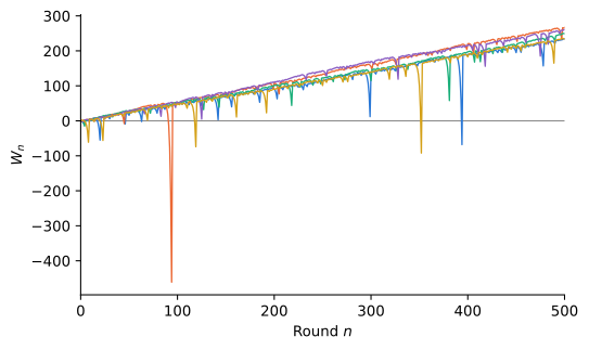
The doubling strategy shows that the value of a martingale at a stopping time need not have the same expectation as its starting value. The gambler stops at a time \tau that is finite with probability one, and W_{\tau} = 1 while W_{0} = 0. What fails is that the losses before \tau are unbounded. The optional stopping theorem below gives a condition that rules this out.

Stopped Processes

A random variable \tau taking values in \{0, 1, 2, \ldots\} \cup \{\infty\} is called a stopping time with respect to \{\mathcal{F}_{n}: 0 \leq n \leq \infty\} if \{\tau \leq n\} \in \mathcal{F}_{n} \text{ for all } 0 \leq n < \infty. If \tau < \infty almost surely, we can define the stopped process Y_{\tau} = \sum_{k = 0}^{\infty} \mathbf{1}_{\{\tau = k\}} Y_{k}. In cases where \operatorname{P}(\tau = \infty) > 0, we can always define the truncated stopping time n \land \tau = \min\{n, \tau\}. The stopped process Y_{n \land \tau} is always well defined.

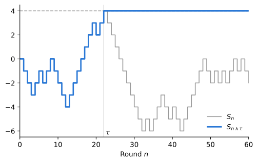
Figure 2 shows a walk stopped at the first time \tau it reaches 4. The stopped process follows the walk up to \tau and stays at S_{\tau} = 4 afterwards, whatever the walk does next.

Figure 2: The figure plots a simple random walk S_{n} (gray) and the stopped process S_{n \land \tau} (blue), where \tau is the first time the walk reaches 4 (dashed).

WarningStopped Martingales are also Martingales

If \{M_{n}\} is a martingale with respect to \{\mathcal{F}_{n}\}, then the stopped process \{M_{n \land \tau}\} is also a martingale with respect to \{\mathcal{F}_{n}\}.

Proof.

We can always write M_{(n + 1) \land \tau} = M_{n + 1} \mathbf{1}_{\{\tau \geq n + 1\}} + M_{n \land \tau} \mathbf{1}_{\{\tau \leq n\}}. Since \mathbf{1}_{\{\tau \geq n + 1\}} = 1 - \mathbf{1}_{\{\tau \leq n\}}, we see that \mathbf{1}_{\{\tau \geq n + 1\}} is \mathcal{F}_{n} measurable. Thus \begin{aligned} \operatorname{E}(M_{n + 1} \mathbf{1}_{\{\tau \geq n + 1\}} \mid \mathcal{F}_{n}) & = \operatorname{E}(M_{n + 1} \mid \mathcal{F}_{n}) \mathbf{1}_{\{\tau \geq n + 1\}} \\ & = M_{n} \mathbf{1}_{\{\tau \geq n + 1\}} \\ & = M_{n \land \tau} \mathbf{1}_{\{\tau \geq n + 1\}}. \end{aligned} Combining this with the decomposition above, \begin{aligned} \operatorname{E}(M_{(n + 1) \land \tau} | \mathcal{F}_{n}) & = \operatorname{E}(M_{n + 1} \mathbf{1}_{\{\tau \geq n + 1\}} \mid \mathcal{F}_{n}) + M_{n \land \tau} \mathbf{1}_{\{\tau \leq n\}} \\ & = M_{n \land \tau} \mathbf{1}_{\{\tau \geq n + 1\}} + M_{n \land \tau} \mathbf{1}_{\{\tau \leq n\}} \\ & = M_{n \land \tau}, \end{aligned} proving that \{M_{n \land \tau}\} is a martingale with respect to \{\mathcal{F}_{n}\}.

Stopping is itself a betting strategy: bet one dollar per round while the game is running and nothing afterwards. With H_{k} = \mathbf{1}_{\{\tau \geq k\}}, M_{n \land \tau} = M_{0} + \sum_{k = 1}^{n} \mathbf{1}_{\{\tau \geq k\}} (M_{k} - M_{k - 1}), and H_{k} is predictable because \{\tau \geq k\} is the complement of \{\tau \leq k - 1\} \in \mathcal{F}_{k - 1}. The result on betting strategies therefore gives a second proof that stopped martingales are martingales.

Optional Stopping

Since \{M_{n \land \tau}\} is a martingale, \operatorname{E}(M_{n \land \tau}) = \operatorname{E}(M_{0}) for every n. If \tau is finite, then M_{n \land \tau} = M_{\tau} as soon as n \geq \tau, so M_{n \land \tau} \to M_{\tau} as n \to \infty. The question is whether the expectations converge too, and the doubling strategy shows that they need not. The following result gives a condition under which they do.

WarningOptional Stopping Theorem

Let \{M_{n}\} be a martingale and \tau a stopping time with respect to \{\mathcal{F}_{n}\}, with \operatorname{P}(\tau < \infty) = 1. If there is a random variable Y with \operatorname{E}(Y) < \infty such that |M_{n \land \tau}| \leq Y for all n, then \operatorname{E}(M_{\tau}) = \operatorname{E}(M_{0}). In particular, the result holds when the stopped process is bounded by a constant.

Proof.

The stopped process converges to M_{\tau} and is dominated by Y, so the dominated convergence theorem gives \operatorname{E}(M_{\tau}) = \operatorname{E}\left(\lim_{n \to \infty} M_{n \land \tau}\right) = \lim_{n \to \infty} \operatorname{E}(M_{n \land \tau}) = \operatorname{E}(M_{0}).

In the doubling strategy, the wealth just before the winning round \tau is -(2^{\tau - 1} - 1), so any Y that dominates the stopped process must be at least 2^{\tau - 1} - 1. Since \operatorname{P}(\tau = k) = 2^{-k}, the expectation of 2^{\tau - 1} is \sum_{k} 2^{k - 1} 2^{-k} = \infty, and no integrable bound exists.

Ruin Probabilities Again

We now revisit the ruin probability problem, previously analyzed using elementary methods, and show how the martingale machinery yields both the ruin probability and the expected duration in a unified way. Consider the simple symmetric random walk: S_{n} = \sum_{i = 1}^{n} X_{i} for n \geq 1, where each X_{i} is an independent fair coin toss, taking values -1 or 1 with probability 1/2. Define the stopping time \tau = \min\{n > 0 : S_{n} = A \text{ or } S_{n} = -B\}, which is measurable with respect to the filtration \mathcal{F}_{n}.

The notes on ruin probabilities show that \tau is finite with probability one and that \operatorname{E}(\tau) < \infty.

The Probability

Recall that S_{n} is a martingale. Since the process stops when it reaches either A or -B, we have |S_{n \land \tau}| \leq \max(A, B) for all n. The stopped process is bounded, so the optional stopping theorem gives \operatorname{E}(S_{\tau}) = S_{0} = 0.

Since we can also write \operatorname{E}(S_{\tau}) = \operatorname{P}(S_{\tau} = A) A + (1 - \operatorname{P}(S_{\tau} = A)) (-B) = 0, we get that \operatorname{P}(S_{\tau} = A) = \frac{B}{A + B}.

The Expectation

Furthermore, since for the simple random walk \operatorname{E}(X_{n}) = 0 and \operatorname{V}(X_{n}) = 1, Example 2 with \sigma^{2} = 1 shows that M_{n} = S_{n}^{2} - n is also a martingale. Because the process stops when it hits A or -B, we have |S_{n \land \tau}| \leq \max(A, B), and therefore |M_{n \land \tau}| = |S_{n \land \tau}^{2} - (n \land \tau)| \leq \max(A^{2}, B^{2}) + \tau. The right-hand side does not depend on n, and it has a finite expectation because \operatorname{E}(\tau) < \infty. The optional stopping theorem therefore gives \operatorname{E}(M_{\tau}) = M_{0} = 0.

Since we also have that \operatorname{E}(M_{\tau}) = A^{2} \frac{B}{A + B} + B^{2} \frac{A}{A + B} - \operatorname{E}(\tau) = 0, we conclude that \operatorname{E}(\tau) = A B.

A Biased Coin

The same method handles a biased coin, where each bet is won with probability p and lost with probability q = 1 - p, with p \neq q. The walk S_{n} is no longer a martingale, so we need a different one. Each factor (q / p)^{X_{i}} is positive with \operatorname{E}\left((q / p)^{X_{i}}\right) = p \frac{q}{p} + q \frac{p}{q} = q + p = 1, so Example 3 shows that Z_{n} = (q / p)^{S_{n}} = \prod_{i = 1}^{n} (q / p)^{X_{i}} is a martingale.

For p > q this martingale has a striking shape, shown in Figure 3 for p = 0.55. By the strong law of large numbers S_{n} / n \to p - q > 0, so S_{n} \to \infty and Z_{n} \to 0 on almost every path, and a typical path falls like (q / p)^{n (p - q)}. Yet \operatorname{E}(Z_{n}) = 1 for every n. The expectation is held up by the rare paths on which the walk is still at or below zero, where Z_{n} \geq 1: after 400 rounds they are 2.5 percent of the paths. Read as wealth, Z_{n} belongs to a gambler who multiplies wealth by q / p with probability p and by p / q with probability q, a fair bet each round, and the typical such gambler is wiped out. A martingale that goes to zero while its expectation stays at one is what the argument without an upper barrier below relies on.

Figure 3: The figure plots 20 simulated paths of the martingale Z_{n} = (q / p)^{S_{n}} for p = 0.55 on a logarithmic scale, together with its expectation, which stays at one (dashed), and the typical path (q / p)^{n (p - q)} (orange).

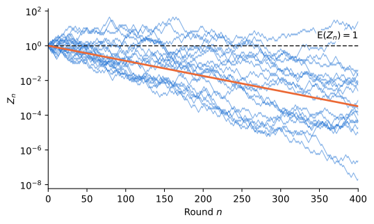
The argument in the notes on ruin probabilities, with (1/2)^{A + B} replaced by p^{A + B}, shows that \tau is finite with probability one and \operatorname{E}(\tau) < \infty. The stopped process Z_{n \land \tau} lies between (q / p)^{-B} and (q / p)^{A}, so it is bounded, and optional stopping gives \operatorname{E}(Z_{\tau}) = Z_{0} = 1. Writing P_{A} = \operatorname{P}(S_{\tau} = A), P_{A} (q / p)^{A} + (1 - P_{A}) (q / p)^{-B} = 1, and solving for P_{A}, P_{A} = \frac{(q / p)^{B} - 1}{(q / p)^{A + B} - 1}, which is the answer the notes on ruin probabilities found by solving a difference equation.

The expected duration follows from a second martingale. The variables X_{i} - (p - q) are independent with mean zero, so Example 1 shows that S_{n} - n (p - q) is a martingale. Its stopped version satisfies |S_{n \land \tau} - (n \land \tau)(p - q)| \leq \max(A, B) + \tau, a bound with finite expectation that does not depend on n, so optional stopping gives \operatorname{E}(S_{\tau}) = (p - q) \operatorname{E}(\tau). Therefore, \operatorname{E}(\tau) = \frac{A P_{A} - B (1 - P_{A})}{p - q}.

The two martingales (q / p)^{S_{n}} and S_{n} - n (p - q) play the roles that S_{n} and S_{n}^{2} - n played for the fair coin. The notes on Poisson processes and Brownian motion follow the same pattern: an exponential martingale gives the ruin probability, with e^{-R} and e^{-2 \mu / \sigma^{2}} in the role of q / p.

No Upper Barrier

Remove the upper barrier, so that the gambler plays until ruined. Let \tau_{B} = \min\{n > 0 : S_{n} = -B\}, with \tau_{B} = \infty on the paths that never reach -B. Now the question is whether the game ends at all.

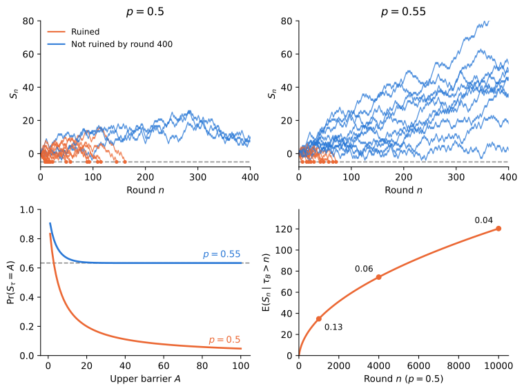
The games with two barriers answer it. The events \{S_{\tau} = A\} shrink as A grows, because a path that reaches A + 1 before -B passes through A first. A path that is ruined climbs only to a finite height before reaching -B, so it is in none of these events once A is large enough. A path that is never ruined reaches every A, because each game with two barriers ends with probability one. Apart from a set of probability zero, the intersection of the events is therefore the event that the gambler is never ruined, and continuity of probability gives \operatorname{P}(\tau_{B} = \infty) = \lim_{A \to \infty} P_{A}. For p > q, (q / p)^{A + B} \to 0 and the limit is 1 - (q / p)^{B} > 0. For the fair coin, the limit is \lim B / (A + B) = 0, and ruin is certain, as in the practice problems on ruin probabilities.

What happens to a gambler who is never ruined? By the strong law of large numbers, S_{n} / n \to p - q, so for p > q the winnings grow without bound, at about p - q per round. The gambler does not wander forever between two levels: in the limit of the games with two barriers, S_{\tau} = A with A = \infty. The fair coin has no such escape. Its walk swings up and down without bound and sooner or later reaches -B, however far up it has gone. Figure 4 shows both cases.

Figure 4: The figure compares a fair coin with a coin won with probability p = 0.55, for a gambler who stops only when ruined at -B = -5 (dashed line in the top panels). The top panels plot 20 simulated paths for each coin over 400 rounds, with ruined paths ending in a dot. The bottom left panel plots the probability of reaching A before -B, which falls to zero for the fair coin and levels off at 1 - (q / p)^{B} (dashed) for the biased one. The bottom right panel plots, for the fair coin, the average winnings of the gamblers not yet ruined after n rounds, computed exactly, with the fraction of gamblers not yet ruined printed next to each dot.

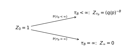
The ruin probability also follows from the martingale Z_{n} = (q / p)^{S_{n}} directly, without the upper barrier, and the argument is the one the notes on Poisson processes use for the insurance ruin problem. Optional stopping does not apply as stated, because \tau_{B} may be infinite, so we work with n \land \tau_{B} instead. The stopped martingale keeps its expectation, and splitting on whether ruin has happened by round n, 1 = \operatorname{E}(Z_{n \land \tau_{B}}) = (q / p)^{-B} \operatorname{P}(\tau_{B} \leq n) + \operatorname{E}(Z_{n} \mathbf{1}_{\{\tau_{B} > n\}}). Let n \to \infty. The first term goes to (q / p)^{-B} \operatorname{P}(\tau_{B} < \infty). In the second, a gambler not yet ruined has S_{n} > -B, so 0 \leq Z_{n} \mathbf{1}_{\{\tau_{B} > n\}} \leq (q / p)^{-B} since q / p < 1. On a path that is ruined the indicator is eventually zero, and on a path that is never ruined S_{n} \to \infty and Z_{n} \to 0, as in Figure 3. The second term therefore goes to zero by dominated convergence, and \operatorname{P}(\tau_{B} < \infty) = (q / p)^{B}. Figure 5 draws the limit as a tree with two branches, like the binomial trees that price options. The martingale starts at one, which is the probability-weighted average of its values on the two branches, and the ruin probability is the weight on the branch where the gambler is ruined. The walk moves one step at a time, so a ruined gambler lands exactly on -B, and the value on that branch is known.

Figure 5: The figure shows the martingale Z_{n} = (q / p)^{S_{n}} stopped at ruin, for p > q. With probability \operatorname{P}(\tau_{B} < \infty) the gambler is ruined and Z_{\tau_{B}} = (q / p)^{-B}; otherwise the winnings grow without bound and Z_{n} goes to zero.

The gamblers who are never ruined drop out of the calculation because the martingale is close to zero where they are: large winnings make (q / p)^{S_{n}} small. The insurance ruin problem has the same structure, with the capital u in place of B and e^{-R} in place of q / p. Premiums exceed expected claims, so a surplus that is never ruined grows without bound, and that is what sends the survivors’ term to zero.

For the fair coin, the same split with the martingale S_{n} gives 0 = \operatorname{E}(S_{n \land \tau_{B}}) = -B \operatorname{P}(\tau_{B} \leq n) + \operatorname{E}(S_{n} \mathbf{1}_{\{\tau_{B} > n\}}). Ruin is certain, so \operatorname{P}(\tau_{B} \leq n) \to 1 and \operatorname{E}(S_{n} \mathbf{1}_{\{\tau_{B} > n\}}) \to B. The survivors’ term does not vanish. Fewer and fewer gamblers remain, but those who do are far ahead: after 10,000 rounds, a fraction 0.04 of the gamblers survive, with average winnings of 120.4 dollars, and the product is close to B = 5. In the limit, S_{\tau_{B}} = -B on every path, so \operatorname{E}(S_{\tau_{B}}) = -B \neq S_{0}, and optional stopping fails. This is the doubling strategy of Example 4 turned around. There, a gain of one dollar is certain and the rare large losses before the first win carry the expectation. Here, a loss of B dollars is certain and the rare large gains before ruin carry it. In both cases no integrable bound dominates the stopped process. It is also why the insurance ruin problem assumes that premiums exceed expected claims: when they are equal, the surplus behaves like the fair coin and ruin is certain.

Practice Problems

Problem 1 Let \{S_{n}\} be the simple symmetric random walk with S_{0} = 0. Which of the following random times are stopping times with respect to \{\mathcal{F}_{n}\}? Explain.

1. The first time \tau that the walk reaches 5.
2. The last time n \leq 10 at which S_{n} = 0.
3. \tau + 1 and \tau - 1, where \tau is the time in the first part.
4. \min(\tau, \rho) and \max(\tau, \rho), where \tau and \rho are any two stopping times.
5. The first time n \leq 10 at which S_{n} equals its maximum over 0 \leq n \leq 10.

Solution

1. Yes. \{\tau \leq n\} = \{\max_{k \leq n} S_{k} \geq 5\} depends only on the first n steps.
2. No. To know that the last visit to 0 was at time 3, we need to know that S_{4}, \ldots, S_{10} are all different from 0, which depends on steps after time 3.
3. \tau + 1 is a stopping time, since \{\tau + 1 \leq n\} = \{\tau \leq n - 1\} \in \mathcal{F}_{n - 1} \subset \mathcal{F}_{n}. \tau - 1 is not: \tau - 1 = 4 means \tau = 5, which happens when the first five steps are all up, and at time 4 the fifth step is unknown. Selling one period before the price reaches a level requires seeing the future.
4. Both are stopping times, since \{\min(\tau, \rho) \leq n\} = \{\tau \leq n\} \cup \{\rho \leq n\} and \{\max(\tau, \rho) \leq n\} = \{\tau \leq n\} \cap \{\rho \leq n\}, and both sets are in \mathcal{F}_{n}. A rule that exits at a take-profit or a stop-loss, whichever comes first, is the minimum of two stopping times.
5. No. Whether time n is the maximum depends on the values after n. Selling at the top is not a strategy anyone can follow.

Problem 2 A gambler bets on a fair coin, where M_{k} - M_{k - 1} = X_{k} is +1 or -1 with probability 1/2, starting from W_{0} = 0. The gambler stakes $1 on the first round and afterwards follows a momentum rule, H_{k} = X_{k - 1} for k \geq 2: bet one dollar that the last move repeats.

1. Show that \{H_{k}\} is predictable, and that \operatorname{E}(W_{n}) = 0.
2. Show that the gains H_{k} X_{k} in different rounds are uncorrelated, and compute \operatorname{V}(W_{n}).
3. A backtest of a trading rule mistakenly uses H_{k} = X_{k}. Compute W_{n}, and explain which assumption of the result on betting strategies fails.

Solution

1. H_{k} = X_{k - 1} is known at time k - 1, and |H_{k}| = 1, so the result on betting strategies applies and \{W_{n}\} is a martingale with \operatorname{E}(W_{n}) = W_{0} = 0.
2. For j < k, H_{j} X_{j} H_{k} is known at time k - 1, so the tower property gives \operatorname{E}(H_{j} X_{j} H_{k} X_{k}) = \operatorname{E}\left(H_{j} X_{j} H_{k} \operatorname{E}(X_{k} \mid \mathcal{F}_{k - 1})\right) = 0. Each gain has mean zero and (H_{k} X_{k})^{2} = 1, so \operatorname{V}(W_{n}) = n. The momentum rule produces exactly the same distribution of gains as betting one dollar on heads every round.
3. W_{n} = \sum_{k = 1}^{n} X_{k}^{2} = n, a sure gain of one dollar per round. The stake H_{k} = X_{k} is not known at time k - 1, so the strategy is not predictable. This is look-ahead bias, as in a backtest that computes a signal from a closing price and then trades at that same closing price.

Problem 3 (★) Let \{S_{n}\} be the simple symmetric random walk with S_{0} = 0. Decide whether each process is a martingale with respect to \{\mathcal{F}_{n}\}.

1. S_{n}^{2}.
2. S_{n}^{3} - 3 n S_{n}.
3. e^{\theta S_{n}} / (\cosh \theta)^{n} for a constant \theta, where \cosh \theta = (e^{\theta} + e^{-\theta})/2.
4. For a biased coin with p \neq q, e^{\theta S_{n}} for a constant \theta. Which values of \theta make it a martingale?

Solution

Each process depends only on the first n steps and is bounded at each n, so the question is whether its conditional expectation one step ahead equals its current value. In each case S_{n + 1} = S_{n} + X_{n + 1}, where X_{n + 1} is independent of \mathcal{F}_{n}.

1. \operatorname{E}(S_{n + 1}^{2} \mid \mathcal{F}_{n}) = S_{n}^{2} + 2 S_{n} \operatorname{E}(X_{n + 1}) + \operatorname{E}(X_{n + 1}^{2}) = S_{n}^{2} + 1, so S_{n}^{2} is not a martingale: it rises by one on average every period. Subtracting n removes the drift, as in Example 2.
2. Using \operatorname{E}(X_{n + 1}) = \operatorname{E}(X_{n + 1}^{3}) = 0 and \operatorname{E}(X_{n + 1}^{2}) = 1, \operatorname{E}(S_{n + 1}^{3} \mid \mathcal{F}_{n}) = S_{n}^{3} + 3 S_{n}^{2} \operatorname{E}(X_{n + 1}) + 3 S_{n} \operatorname{E}(X_{n + 1}^{2}) + \operatorname{E}(X_{n + 1}^{3}) = S_{n}^{3} + 3 S_{n}. Also \operatorname{E}(3 (n + 1) S_{n + 1} \mid \mathcal{F}_{n}) = 3 (n + 1) S_{n}, so \operatorname{E}(S_{n + 1}^{3} - 3 (n + 1) S_{n + 1} \mid \mathcal{F}_{n}) = S_{n}^{3} - 3 n S_{n}, and the process is a martingale.
3. e^{\theta S_{n}} / (\cosh \theta)^{n} = \prod_{i = 1}^{n} e^{\theta X_{i}} / \cosh \theta. Each factor is positive with \operatorname{E}(e^{\theta X_{i}}) / \cosh \theta = \frac{1}{2} (e^{\theta} + e^{-\theta}) / \cosh \theta = 1, so Example 3 shows that the product is a martingale.
4. \operatorname{E}(e^{\theta S_{n + 1}} \mid \mathcal{F}_{n}) = e^{\theta S_{n}} (p e^{\theta} + q e^{-\theta}), so we need p e^{\theta} + q e^{-\theta} = 1. With z = e^{\theta} this is p z^{2} - z + q = 0, with roots z = 1 and z = q / p. The constant \theta = 0 gives a trivial martingale, and \theta = \ln(q / p) gives (q / p)^{S_{n}}, the martingale used in the notes for the biased coin.

Problem 4 (★) Let Y be a random variable with \operatorname{E}(|Y|) < \infty, and define M_{n} = \operatorname{E}(Y \mid \mathcal{F}_{n}).

1. Show that \{M_{n}\} is a martingale.
2. Let \{S_{n}\} be the simple symmetric random walk with S_{0} = 0, let N be a fixed time, and let Y = S_{N}^{2}. Show that M_{n} = S_{n}^{2} + (N - n) for n \leq N.
3. Use the previous problem to show that \operatorname{E}(S_{N}^{3} \mid \mathcal{F}_{n}) = S_{n}^{3} + 3 (N - n) S_{n} for n \leq N.
4. With a zero interest rate, the price at time n of a claim that pays Y at time N is \operatorname{E}^{*}(Y \mid \mathcal{F}_{n}), an expectation under a risk-neutral probability \operatorname{P}^{*}. Explain why no strategy of buying and selling the claim has a positive expected profit under \operatorname{P}^{*}.

Solution

1. Since \mathcal{F}_{n} \subset \mathcal{F}_{n + 1}, the tower property gives \operatorname{E}(M_{n + 1} \mid \mathcal{F}_{n}) = \operatorname{E}\left(\operatorname{E}(Y \mid \mathcal{F}_{n + 1}) \mid \mathcal{F}_{n}\right) = \operatorname{E}(Y \mid \mathcal{F}_{n}) = M_{n}. The forecast of Y is revised as information arrives, but the revisions cannot be predicted.
2. Write S_{N} = S_{n} + D, where D = X_{n + 1} + \cdots + X_{N} is independent of \mathcal{F}_{n}, with mean zero and variance N - n. Then \operatorname{E}(S_{N}^{2} \mid \mathcal{F}_{n}) = S_{n}^{2} + 2 S_{n} \operatorname{E}(D) + \operatorname{E}(D^{2}) = S_{n}^{2} + (N - n). This is the martingale S_{n}^{2} - n of Example 2 plus the constant N.
3. Since S_{n}^{3} - 3 n S_{n} and S_{n} are martingales, \operatorname{E}(S_{N}^{3} - 3 N S_{N} \mid \mathcal{F}_{n}) = S_{n}^{3} - 3 n S_{n} and \operatorname{E}(S_{N} \mid \mathcal{F}_{n}) = S_{n}. Adding 3 N S_{n} to both sides of the first equation gives the result.
4. By the first part, the price P_{n} = \operatorname{E}^{*}(Y \mid \mathcal{F}_{n}) is a martingale under \operatorname{P}^{*}. Holding H_{k} units of the claim from k - 1 to k gives the martingale transform \sum_{k} H_{k} (P_{k} - P_{k - 1}), which has zero expectation under \operatorname{P}^{*} for any predictable bounded \{H_{k}\}.

Problem 5 (★) A gambler follows the doubling strategy of Example 4 but can lose at most 2^{m} - 1 dollars, so the gambler stops at the first win or after m losses in a row, whichever comes first.

1. Show that with a fair coin the gambler wins one dollar with probability 1 - 2^{-m} and otherwise loses 2^{m} - 1 dollars. Compute both numbers for m = 10, and check that the expected gain is zero.
2. Explain why the optional stopping theorem applies to this strategy but not to the doubling strategy without a limit.
3. In roulette each bet wins with probability p = 18/38. Show that the expected gain is 1 - (2 q)^{m}, and compute it for m = 10.
4. Show that the expected total amount wagered is \left((2 q)^{m} - 1\right) / (2 q - 1), and interpret the expected loss.

Solution

1. The gambler loses all m rounds with probability 2^{-m}, losing 1 + 2 + \cdots + 2^{m - 1} = 2^{m} - 1 dollars, and otherwise wins one dollar, as in Example 4. For m = 10, the gambler wins a dollar with probability 0.999 and loses $1,023 with probability 0.001. The expected gain is (1 - 2^{-m}) - 2^{-m} (2^{m} - 1) = 0.
2. The stopping time is at most m, and the wealth stays between -(2^{m} - 1) and 1, so the stopped process is bounded and optional stopping gives \operatorname{E}(W_{\tau}) = W_{0} = 0. Without a limit, the losses before the first win are unbounded, and the notes show that no integrable bound exists.
3. The gambler loses all m rounds with probability q^{m}, so the expected gain is (1 - q^{m}) - q^{m} (2^{m} - 1) = 1 - (2 q)^{m}. With 2 q = 40/38 and m = 10, this is 1 - 1.670 = -0.670 dollars.
4. The stake 2^{k - 1} on round k is placed only if the first k - 1 rounds were lost, which happens with probability q^{k - 1}. The expected amount wagered is \sum_{k = 1}^{m} 2^{k - 1} q^{k - 1} = \sum_{k = 1}^{m} (2 q)^{k - 1} = \frac{(2 q)^{m} - 1}{2 q - 1}, which is 0.670 \times 19 = 12.73 dollars for m = 10. Since 2 q - 1 = q - p = 1/19, the expected loss is the house edge times the expected amount wagered, as for any strategy. Doubling does not avoid the edge; it raises the amount wagered.

Problem 6 (★) A stock trades at $100, and over each of two periods its price rises by 20% or falls by 10%. The interest rate is zero. A call option pays C = \max(S_{2} - 100, 0) at time 2. Under a risk-neutral probability \operatorname{P}^{*} the price rises with probability p^{*} each period, independently across periods.

1. Find the p^{*} that makes \{S_{n}\} a martingale under \operatorname{P}^{*}.
2. The price of the call at time n is C_{n} = \operatorname{E}^{*}(C \mid \mathcal{F}_{n}). Compute C_{1} after each move and C_{0}.
3. The fifth practice problem on conditioning and independence found \operatorname{E}(C) = 19.68 when the price rises with probability 0.6. Why is the price of the call so much lower?
4. Let H_{1} = (C_{1}^{u} - C_{1}^{d}) / (S_{1}^{u} - S_{1}^{d}), where the superscripts denote the values after an up and a down move. Show that C_{1} = C_{0} + H_{1} (S_{1} - S_{0}) after each move. Compute H_{2} in the same way at each node at time 1, and check that C_{2} = C_{0} + \sum_{k = 1}^{2} H_{k} (S_{k} - S_{k - 1}) on the path that goes up and then down.

Solution

1. We need \operatorname{E}^{*}(S_{n + 1} \mid \mathcal{F}_{n}) = S_{n} (1.2 p^{*} + 0.9 (1 - p^{*})) = S_{n}, so 0.9 + 0.3 p^{*} = 1 and p^{*} = 1/3.
2. The payoffs are 44 after two up moves, 8 after one up and one down move in either order, and 0 after two down moves. After an up move, C_{1}^{u} = \frac{1}{3} (44) + \frac{2}{3} (8) = 20, and after a down move, C_{1}^{d} = \frac{1}{3} (8) + \frac{2}{3} (0) = 2.67. By the tower property, C_{0} = \frac{1}{3} (20) + \frac{2}{3} (2.67) = 8.44.
3. Under \operatorname{P}^{*} the stock earns the interest rate, zero, while under the probability 0.6 it earns 0.6 (20\%) + 0.4 (-10\%) = 8\% per period. The expected payoff of 19.68 includes the reward for bearing the risk of the stock, and the price does not. The probability p^{*} is chosen to price the stock correctly, and it is not a forecast.
4. H_{1} = (20 - 2.67) / (120 - 90) = 0.578 shares. After an up move, C_{0} + H_{1} (20) = 8.44 + 11.56 = 20 = C_{1}^{u}, and after a down move, C_{0} + H_{1} (-10) = 8.44 - 5.78 = 2.67 = C_{1}^{d}. At time 1, H_{2} = (44 - 8) / (144 - 108) = 1 after an up move and H_{2} = (8 - 0)/(108 - 81) = 0.296 after a down move. On the path up then down, C_{0} + H_{1} (20) + 1 \times (108 - 120) = 20 - 12 = 8, the payoff. The call price is a martingale transform of the stock price: a predictable strategy in the stock replicates the call, and its martingale property is why the price is an expectation under \operatorname{P}^{*}.

Problem 7 (★★) Let X_{1}, X_{2}, \ldots be iid with mean \mu and |X_{i}| \leq c, let S_{n} = X_{1} + \cdots + X_{n}, and let \tau be a stopping time with \operatorname{E}(\tau) < \infty.

1. Use the martingale S_{n} - n \mu and the optional stopping theorem to prove Wald’s identity, \operatorname{E}(S_{\tau}) = \mu \operatorname{E}(\tau).
2. Each trial in a sequence succeeds with probability p, independently. Use Wald’s identity to show that the expected number of trials until the first success is 1 / p.
3. For the simple symmetric random walk, let \tau_{1} = \min\{n > 0 : S_{n} = 1\}, which is finite with probability one by the practice problems on ruin probabilities. Show that \operatorname{E}(\tau_{1}) = \infty.

Solution

1. By Example 1, S_{n} - n \mu is a martingale, since the X_{i} - \mu are independent with mean zero. Its stopped version satisfies |S_{n \land \tau} - (n \land \tau) \mu| \leq \sum_{k = 1}^{n \land \tau} |X_{k} - \mu| \leq (c + |\mu|) \tau, a bound that does not depend on n and has finite expectation. Optional stopping gives \operatorname{E}(S_{\tau} - \tau \mu) = 0.
2. Let X_{i} = 1 if trial i succeeds and 0 otherwise, so \mu = p, and let \tau be the first success. Then \operatorname{P}(\tau > n) = (1 - p)^{n}, so \operatorname{E}(\tau) = \sum_{n} \operatorname{P}(\tau > n) = 1 / p is finite, as Wald’s identity requires. Since S_{\tau} = 1, Wald’s identity gives 1 = p \operatorname{E}(\tau), so \operatorname{E}(\tau) = 1 / p.
3. If \operatorname{E}(\tau_{1}) were finite, Wald’s identity with \mu = 0 would give 1 = \operatorname{E}(S_{\tau_{1}}) = 0 \times \operatorname{E}(\tau_{1}) = 0. The fair walk is sure to gain a dollar eventually, but the expected wait is infinite, which is the reason the doubling strategy needs unlimited credit.

Problem 8 (★★) Let \{S_{n}\} be the simple symmetric random walk with S_{0} = 0, let A \geq 1 be an integer, and let \tau = \min\{n > 0 : |S_{n}| = A\}. By the third problem, M_{n} = e^{\theta S_{n}} / (\cosh \theta)^{n} is a martingale for every \theta.

1. Show that |M_{n \land \tau}| \leq e^{|\theta| A}, and use optional stopping with \theta and with -\theta to show that \operatorname{E}\left((\cosh \theta)^{-\tau}\right) \cosh(\theta A) = 1.
2. Set z = 1 / \cosh \theta to show that the probability generating function of \tau is G_{\tau}(z) = 1 / \cosh(\theta A). Check the answer for A = 1, and for A = 2 against G_{\tau}(z) = z^{2} / (2 - z^{2}) from the practice problems on ruin probabilities.
3. Expand both sides of the first part to second order in \theta to show that \operatorname{E}(\tau) = A^{2}.

Solution

1. Before \tau the walk stays in [-A, A], so e^{\theta S_{n \land \tau}} \leq e^{|\theta| A}, and \cosh \theta \geq 1. The stopped martingale is bounded and \tau is finite, so optional stopping gives \operatorname{E}\left(e^{\theta S_{\tau}} (\cosh \theta)^{-\tau}\right) = M_{0} = 1. The same holds with -\theta in place of \theta. Averaging the two equations, \operatorname{E}\left(\cosh(\theta S_{\tau}) (\cosh \theta)^{-\tau}\right) = 1, and \cosh(\theta S_{\tau}) = \cosh(\theta A) because S_{\tau} = \pm A and \cosh is even.
2. As \theta ranges over [0, \infty), z = 1 / \cosh \theta ranges over (0, 1], and \operatorname{E}(z^{\tau}) = 1 / \cosh(\theta A). For A = 1, G_{\tau}(z) = z, so \tau = 1, as it must be. For A = 2, \cosh(2 \theta) = 2 \cosh^{2} \theta - 1 = 2 / z^{2} - 1, so G_{\tau}(z) = z^{2} / (2 - z^{2}).
3. For small \theta, \cosh \theta = 1 + \frac{1}{2} \theta^{2} + \cdots, so (\cosh \theta)^{-\tau} = e^{-\tau \ln \cosh \theta} = 1 - \frac{1}{2} \tau \theta^{2} + \cdots and 1 / \cosh(\theta A) = 1 - \frac{1}{2} A^{2} \theta^{2} + \cdots. The first part says that the expectation of the first expansion equals the second, and matching the \theta^{2} terms gives \operatorname{E}(\tau) = A^{2}, which is AB with A = B.