Recursive Preferences in a Multiperiod Economy

Introduction

The SDFs of Multiperiod Asset Pricing and Intertemporal Portfolio Choice come from time-separable utility, where a single curvature parameter sets both risk aversion and the elasticity of intertemporal substitution. The Epstein-Zin preferences notebook separated the two in a two-date setting, by guessing a homothetic consumption rule and solving a single maximization problem. That argument is clean but sidesteps the recursion that defines these preferences, and the recursion is what makes them useful when there are many periods.

This notebook derives the SDF directly from the multiperiod recursion. A perturbation argument gives the SDF for any Kreps-Porteus aggregator in terms of the utility process. For Epstein-Zin preferences, Euler’s theorem for homogeneous functions then translates utility into total wealth, and the SDF becomes a function of consumption growth and the return on wealth, valid at every date. A map of the weight \theta across preference parameters shows where the calibrations used in the literature sit. Finally, with i.i.d. investment opportunities the wealth return drops out of risk premia, which shows that the separation of risk aversion from intertemporal substitution matters for risk premia only when opportunities vary over time.

General Recursive Utility

Kreps and Porteus (1978) develop a framework for recursive utility that separates attitudes toward risk from the willingness to substitute consumption over time. A general Kreps-Porteus aggregator takes the form V_t = U(C_t, \mu_t), where U(C, \mu) is an increasing aggregator and \mu_t is the certainty equivalent of next-period utility under a von Neumann-Morgenstern risk aggregator: \mu_t = \phi^{-1}\!\left(\operatorname{E}_t\!\left[\phi(V_{t+1})\right]\right), for some increasing, concave \phi. The concavity of \phi makes the agent averse to uncertainty about future utility levels, while the curvature of U in its first argument separately controls the willingness to substitute consumption across time. This is the key departure from standard expected utility, where a single function governs both simultaneously. Epstein-Zin preferences (Epstein and Zin 1989), the subject of the next section, are the leading special case.

Kreps, David M., and Evan L. Porteus. 1978. “Temporal Resolution of Uncertainty and Dynamic Choice Theory.” Econometrica 46 (1): 185–200.

Epstein, Larry G., and Stanley E. Zin. 1989. “Substitution, Risk Aversion, and the Temporal Behavior of Consumption and Asset Returns: A Theoretical Framework.” Econometrica 57 (4): 937–69.

¹ The perturbation changes only C_t and C_{t+1}, so \mu_{t+1}, which depends on consumption from t+2 onward, is unaffected and \partial V_{t+1}/\partial \xi = U_c(C_{t+1}, \mu_{t+1})\,X_{t+1}. Differentiating \mu_t = \phi^{-1}(\operatorname{E}_t[\phi(V_{t+1})]) gives \partial \mu_t/\partial \xi = \operatorname{E}_t[\phi'(V_{t+1})\,U_c(C_{t+1},\mu_{t+1})\,X_{t+1}]/\phi'(\mu_t), and the chain rule through U(C_t - \xi P_t, \mu_t) multiplies this by U_\mu and sets it equal to P_t U_c.

² Other risk aggregators give other adjustments. The entropic \phi(v) = -e^{-\alpha v} gives e^{-\alpha(V_{t+1}-\mu_t)}, the form behind robust control and multiplier preferences.

To derive the SDF, consider a small perturbation in the consumption plan: give up \xi\,P_t units of consumption today in exchange for \xi\,X_{t+1} units tomorrow. At the optimum the agent is indifferent at the margin, so the derivative of V_t = U(C_t - \xi P_t,\, \mu_t(\xi)) with respect to \xi vanishes at \xi = 0. This gives the first-order condition¹ P_t\,U_c(C_t,\mu_t) = U_\mu(C_t,\mu_t)\, \frac{\operatorname{E}_t\!\left[\phi'(V_{t+1})\,U_c(C_{t+1},\mu_{t+1})\,X_{t+1}\right]}{\phi'(\mu_t)}, so the SDF is M_{t+1} = \underbrace{\frac{U_\mu(C_t,\mu_t)}{U_c(C_t,\mu_t)}}_{\text{aggregator ratio}} \cdot \underbrace{\frac{\phi'(V_{t+1})}{\phi'(\mu_t)}}_{\text{risk adjustment}} \cdot \underbrace{U_c(C_{t+1},\mu_{t+1})}_{\text{marginal utility}}. \tag{1} The first and last factors are the ones time-separable utility already has: the rate at which the aggregator trades current consumption for continuation utility, and the marginal utility of consumption next period. The middle factor is new. It compares realized utility to the certainty equivalent through the lens of \phi, so the SDF is high in states where continuation utility turns out low. For power \phi(v) = v^{1-\gamma}/(1-\gamma) it is (V_{t+1}/\mu_t)^{-\gamma}.² With the additive aggregator U(C,\mu) = u(C) + \beta\mu and a linear \phi, the factor is one and (1) reduces to the time-separable SDF \beta u'(C_{t+1})/u'(C_t).

Epstein-Zin Preferences

The agent has preferences over consumption streams (C_t, C_{t+1}, C_{t+2},\ldots) of the Kreps-Porteus form V_t = U(C_t, \mu_t), with aggregator U(C,\mu) = [(1-\beta)C^{1-1/\psi} + \beta\mu^{1-1/\psi}]^{1/(1-1/\psi)} and power risk aggregator \phi(v) = v^{1-\gamma}/(1-\gamma), so the certainty equivalent is \mu_t = \left[\operatorname{E}_t\!\left(V_{t+1}^{1-\gamma}\right)\right]^{\!1/(1-\gamma)}. The parameters \beta\in(0,1), \gamma>0, and \psi>0 are the time-discount factor, coefficient of relative risk aversion, and elasticity of intertemporal substitution. The aggregator takes the explicit form V_t = \left[(1-\beta)\,C_t^{1-1/\psi} + \beta\,\mu_t^{1-1/\psi}\right]^{1/(1-1/\psi)}, \tag{2} or equivalently, V_t^{1-1/\psi} = (1-\beta)\,C_t^{1-1/\psi} + \beta\,\mu_t^{1-1/\psi}. \tag{3} When \psi = 1/\gamma the aggregator collapses to standard CRRA utility with coefficient \gamma.

Homotheticity and the Wealth Identity

The aggregator (2) is linearly homogeneous in consumption: scaling consumption at every date and in every state by \lambda > 0 scales V_t by \lambda, because the certainty equivalent \mu_t is itself homogeneous of degree one. Euler’s theorem for homogeneous functions then says that V_t equals the sum of its derivatives times their arguments, summed over all future dates t+\tau and states s: V_t = \sum_{\tau=0}^{\infty} \sum_{s} \frac{\partial V_t}{\partial C_{t+\tau}(s)}\,C_{t+\tau}(s). Each derivative, divided by U_c(C_t,\mu_t), is the marginal rate of substitution between consumption today and consumption in state s at t+\tau. By the perturbation argument above, it is the price at t of a claim paying one unit in that state, which is the probability of the state times the compounded SDF M_{t,t+\tau} of Multiperiod Asset Pricing, with M_{t,t} = 1.³ Dividing by U_c(C_t,\mu_t) therefore turns the right-hand side into the value of the entire consumption stream, including current consumption, which is total wealth W_t: \frac{V_t}{U_c(C_t,\mu_t)} = \operatorname{E}_t\!\left[\sum_{\tau=0}^{\infty} M_{t,t+\tau}\,C_{t+\tau}\right] = W_t. \tag{4}

³ Under time-separable utility M_{t,t+\tau} is the ratio of marginal utilities \beta^\tau u'(C_{t+\tau})/u'(C_t). Under Epstein-Zin preferences it is the product of the one-period SDFs (1) between t and t+\tau, each of which carries a risk adjustment \phi'(V)/\phi'(\mu) that does not telescope. The ratio U_c(C_{t+\tau},\mu_{t+\tau})/U_c(C_t,\mu_t) alone would leave those adjustments out.

Substituting U_c(C_t,\mu_t) = (1-\beta)\,C_t^{-1/\psi}\,V_t^{1/\psi} into V_t = U_c(C_t,\mu_t)\,W_t and collecting the powers of V_t, V_t^{1-1/\psi} = (1-\beta)\,C_t^{-1/\psi}\,W_t. \tag{5} The entire infinite-dimensional consumption stream is thus compressed into two quantities: current consumption C_t and total wealth W_t.

The Certainty Equivalent

The recursion (3) splits V_t^{1-1/\psi} into a current term (1-\beta)C_t^{1-1/\psi} = (1-\beta)C_t^{-1/\psi}\cdot C_t and a future term \beta\mu_t^{1-1/\psi}. Subtracting the current term from (5) leaves \beta\,\mu_t^{1-1/\psi} = (1-\beta)\,C_t^{-1/\psi}\,(W_t - C_t). \tag{6} The certainty equivalent of future utility is pinned down by savings W_t - C_t, which are invested and grow to next-period wealth W_{t+1} = R^w_{t+1}(W_t - C_t), where R^w_{t+1} is the gross return on the wealth portfolio. Dividing (5) at t+1 by (6), \left(\frac{V_{t+1}}{\mu_t}\right)^{1-1/\psi} = \beta\,R^w_{t+1}\left(\frac{C_{t+1}}{C_t}\right)^{-1/\psi}. \tag{7} The surprise in continuation utility, realized utility relative to its certainty equivalent, depends only on the wealth return and consumption growth.

Deriving the Pricing Kernel

We apply (1) to the Epstein-Zin aggregator, whose partial derivatives are U_c = (1-\beta)\,C^{-1/\psi}\,U^{1/\psi}, \qquad U_\mu = \beta\,\mu^{-1/\psi}\,U^{1/\psi}, together with \phi'(v) = v^{-\gamma}. The aggregator ratio is U_\mu/U_c = \beta\mu_t^{-1/\psi}/\bigl((1-\beta)C_t^{-1/\psi}\bigr), the risk adjustment is (V_{t+1}/\mu_t)^{-\gamma}, and marginal utility next period is (1-\beta)C_{t+1}^{-1/\psi}V_{t+1}^{1/\psi}. Multiplying the three factors, M_{t+1} = \beta\!\left(\frac{C_{t+1}}{C_t}\right)^{\!-1/\psi} \left(\frac{V_{t+1}}{\mu_t}\right)^{\!1/\psi-\gamma}. \tag{8} This is an exact expression for the SDF in terms of the utility process, and (7) translates it into observables. Define \theta = \frac{1-\gamma}{1-1/\psi}, \qquad\text{so that}\qquad \frac{1/\psi-\gamma}{1-1/\psi} = \theta - 1. Raising (7) to the power \theta - 1 and substituting into (8), the Epstein-Zin stochastic discount factor is M_{t+1} = \beta\!\left(\frac{C_{t+1}}{C_t}\right)^{\!-1/\psi} \left[\beta\,R_{t+1}^w\left(\frac{C_{t+1}}{C_t}\right)^{\!-1/\psi}\right]^{\theta-1} = \beta^\theta \left(\frac{C_{t+1}}{C_t}\right)^{\!-\theta/\psi} (R_{t+1}^w)^{\theta-1}, \tag{9} or equivalently, M_{t+1} = \left[\beta\!\left(\frac{C_{t+1}}{C_t}\right)^{\!-1/\psi}\right]^{\!\theta} \left[\frac{1}{R_{t+1}^w}\right]^{\!1-\theta}, \qquad \theta = \frac{1-\gamma}{1-1/\psi}. \tag{10} The parameter \theta measures the weight placed on the consumption-growth factor relative to the wealth-return factor. When \theta = 1, which occurs exactly when \psi = 1/\gamma (the CRRA case), the wealth return drops out entirely. When \theta \neq 1, the wealth return enters the SDF as a separate pricing factor, reflecting the agent’s concern for news about future investment opportunities beyond what current consumption growth reveals. The further \theta departs from one, the more the wealth return matters as an independent pricing factor, provided investment opportunities vary over time, as the next section shows.

For an individual investor, R^w_{t+1} is the return on that investor’s own wealth. With a representative investor, wealth is the claim to aggregate consumption, and R^w_{t+1} is the return on that claim. This is why later notebooks call it the market return, and why empirical work proxies it with the return on a broad stock index.

Figure 1 shows how \theta depends on the two preference parameters. The CRRA curve \psi = 1/\gamma is the only place where \theta = 1, and it also separates the agents who prefer early resolution of uncertainty, \gamma > 1/\psi, from those who prefer late resolution.

Figure 1: The weight \theta = (1-\gamma)/(1-1/\psi) across preference parameters, on logarithmic scales. The black curve is CRRA utility, \psi = 1/\gamma, where \theta = 1. The hatched area above it is where the agent prefers early resolution of uncertainty. The dashed line \psi = 1 is where \theta is undefined.

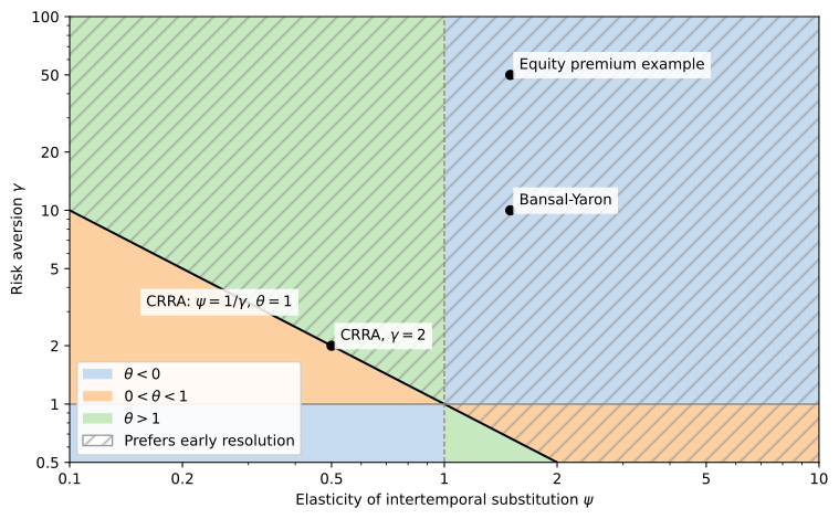
The calibrations used in the literature sit in the upper right quadrant, with \gamma > 1 and \psi > 1. There \theta < 0, so the wealth return enters the SDF with a weight 1 - \theta greater than one: the Bansal-Yaron calibration has \theta = -27, and the equity premium example of Lognormal Consumption Growth has \theta = -147. The map also shows that preferring early resolution does not by itself put an agent in that quadrant. Above the CRRA curve, \theta can be negative, between zero and one, or greater than one, depending on which side of \gamma = 1 and \psi = 1 the agent lies.

Constant Investment Opportunities

Suppose investment opportunities are i.i.d. over time. The agent then faces the same problem at every date, scaled by wealth, and homotheticity of the aggregator implies that the optimal portfolio and the consumption-wealth ratio are constant, C_t = k W_t, so the wealth return R^w_{t+1} is i.i.d. as well. Wealth evolves as W_{t+1} = R^w_{t+1}(W_t - C_t) = R^w_{t+1}(1-k)W_t, so consumption growth is proportional to the wealth return: \frac{C_{t+1}}{C_t} = \frac{W_{t+1}}{W_t} = (1-k)\,R^w_{t+1}. \tag{11} Substituting (11) into (9) to eliminate the wealth return, and using -\theta/\psi + \theta - 1 = \theta(1-1/\psi) - 1 = -\gamma, M_{t+1} = \beta^\theta (1-k)^{1-\theta} \left(\frac{C_{t+1}}{C_t}\right)^{\!-\gamma}. \tag{12} Eliminating consumption growth instead gives M_{t+1} = \beta^\theta (1-k)^{-\theta/\psi}\,(R^w_{t+1})^{-\gamma}.

Either way the SDF is a single power with exponent -\gamma. It is the CRRA SDF with risk aversion \gamma, with the discount factor \beta replaced by the constant \beta^\theta (1-k)^{1-\theta}. The two factors in (10) are perfectly correlated, so the wealth return carries no information beyond consumption growth. Since a constant scaling of the SDF cancels from \operatorname{E}_t[M_{t+1}(R^i_{t+1} - R^f_{t+1})] = 0, risk premia are exactly those of a CRRA investor with risk aversion \gamma, whatever the value of \psi. The elasticity of intertemporal substitution matters only through the constant, which together with k sets the level of the risk-free rate, 1/R^f = \beta^\theta (1-k)^{1-\theta}\,\operatorname{E}[(C_{t+1}/C_t)^{-\gamma}]. Lognormal Consumption Growth works out that dependence explicitly.

A separately priced wealth return, and with it a separation of \gamma from \psi in risk premia, therefore requires time-varying investment opportunities, so that news about future returns moves the wealth return without moving current consumption one for one.

Where This Leads

The SDF (10) is exact, but it prices assets with the return on total wealth, which is not observed, and its second factor matters only when investment opportunities change. The following notebooks work out what that means in practice. Lognormal Consumption Growth takes logs of (10) under joint normality, which turns it into closed forms for the risk-free rate and for risk premia as a combination of consumption and wealth-return covariances. Risk Premia in Intertemporal Models then log-linearizes the budget constraint to express the wealth return through news about future returns and consumption growth, the terms that vanish in the i.i.d. case above. Recursive Utility in Continuous Time builds the continuous-time counterpart through stochastic differential utility and reaches the same conclusion: with a constant opportunity set, \psi affects only the consumption-wealth ratio and the risk-free rate.