Multiperiod Asset Pricing

Introduction

The consumption-based asset pricing notebook priced a payoff X received one period ahead, P = \operatorname{E}(MX) with M = \beta u'(C_1)/u'(C_0). Most assets do not fit that mold. A stock pays dividends for as long as the firm exists, a bond pays coupons until it matures, and an option pays at a date that may be years away. Pricing such claims requires discounting cash flows that arrive at many different dates, each with its own risk.

This notebook extends the two-date framework to an infinite horizon with time-separable utility. We first derive the one-period Euler equation at every date, now with dividends and resale prices, and then iterate it forward to price any stream of cash flows. The iteration produces a discount factor for each horizon, which we use to read off the term structure of real interest rates and the risk adjustment applied to each cash flow. A numerical example with three scenarios puts the pieces together, and an economy with persistent expected growth then extends it to whole yield curves and to the pricing of a stock.

The One-Period Euler Equation

Consider an investor who ranks consumption streams \{C_{t+j}\}_{j=0}^{\infty} by time-separable expected utility, V_t = \operatorname{E}_t \sum_{j=0}^{\infty} \beta^{j} u(C_{t+j}). \tag{1} Separating the first term and applying the law of iterated expectations to the rest gives a recursive form: \begin{aligned} V_t &= u(C_t) + \beta \operatorname{E}_t \sum_{j=0}^{\infty} \beta^{j} u(C_{t+1+j}) \\ &= u(C_t) + \beta \operatorname{E}_t \operatorname{E}_{t+1} \sum_{j=0}^{\infty} \beta^{j} u(C_{t+1+j}) \\ &= u(C_t) + \beta \operatorname{E}_t V_{t+1}. \end{aligned} \tag{2} Lifetime utility is current felicity plus the discounted expected value of the same object one period later. The recursion is what makes a one-period argument enough.

Suppose the investor follows an optimal plan and consider a small deviation from it. At date t the investor buys \xi additional units of an asset with ex-dividend price P_t,¹ and at t+1 collects the dividend D_{t+1} and sells the units at P_{t+1}. Consumption falls by \xi P_t at t, rises by \xi(P_{t+1} + D_{t+1}) at t+1, and is unchanged afterward. By (2), the deviation affects only u(C_t) and the first term of V_{t+1}: u(C_t - \xi P_t) + \beta \operatorname{E}_t\!\left[u\bigl(C_{t+1} + \xi(P_{t+1} + D_{t+1})\bigr)\right] + \text{terms independent of } \xi. Since the plan is optimal, the derivative with respect to \xi vanishes at \xi = 0: P_t = \operatorname{E}_t\!\left[M_{t,t+1}\,(P_{t+1} + D_{t+1})\right], \qquad M_{t,t+1} = \beta\frac{u'(C_{t+1})}{u'(C_t)}. \tag{3} This is the Euler equation of the two-date model, with the payoff now made up of next period’s dividend and resale price. Dividing by P_t gives the familiar return form \operatorname{E}_t[M_{t,t+1} R_{t+1}] = 1 with R_{t+1} = (P_{t+1} + D_{t+1})/P_t. The same condition holds at every date, because the investor faces the same kind of decision at every date.²

¹ The price P_t is quoted after the date-t dividend has been paid, so a buyer at t is entitled to D_{t+1} and later dividends but not to D_t. That is why the payoff one period later is P_{t+1} + D_{t+1}.

² Later notebooks use only the one-period SDF and write it as M_{t+1} \equiv M_{t,t+1}. Both dates are needed here because the argument compounds one-period factors into M_{t,t+j}, whose start and end dates must link up.

From One Period to Many

Equation (3) links today’s price to tomorrow’s. Substituting the same equation for P_{t+1} and applying the law of iterated expectations links it to the price two periods ahead: \begin{aligned} P_t &= \operatorname{E}_t\!\left[M_{t,t+1} D_{t+1}\right] + \operatorname{E}_t\!\left[M_{t,t+1}\,\operatorname{E}_{t+1}\!\left[M_{t+1,t+2}(P_{t+2} + D_{t+2})\right]\right] \\ &= \operatorname{E}_t\!\left[M_{t,t+1} D_{t+1} + M_{t,t+1} M_{t+1,t+2} D_{t+2}\right] + \operatorname{E}_t\!\left[M_{t,t+1} M_{t+1,t+2} P_{t+2}\right]. \end{aligned} Each substitution adds one dividend, discounted by the product of the one-period SDFs up to its payment date. Define the compounded SDF from t to t+j as that product: M_{t,t+j} = \prod_{i=1}^{j} M_{t+i-1,\,t+i} = \prod_{i=1}^{j} \beta\frac{u'(C_{t+i})}{u'(C_{t+i-1})}. \tag{4} After T substitutions, P_t = \operatorname{E}_t \sum_{j=1}^{T} M_{t,t+j}\, D_{t+j} + \operatorname{E}_t\!\left[M_{t,t+T}\, P_{t+T}\right]. \tag{5}

The ratios of marginal utilities in (4) telescope, whatever the utility function: M_{t,t+j} = \beta^j \cdot \frac{u'(C_{t+1})}{u'(C_t)} \cdot \frac{u'(C_{t+2})}{u'(C_{t+1})} \cdots \frac{u'(C_{t+j})}{u'(C_{t+j-1})} = \beta^j \frac{u'(C_{t+j})}{u'(C_t)}. \tag{6} The intermediate consumption levels cancel, so the discount factor for horizon j depends only on marginal utility at the two ends.³

³ The same result follows directly from a perturbation that spans j periods. Buying a claim at t and holding it until t+j transfers consumption from t to t+j, and at the optimum the price of that transfer is the marginal rate of substitution \beta^j u'(C_{t+j})/u'(C_t). Rolling over one-period claims and holding a single long-dated claim are two ways of moving consumption across the same dates, and they must be priced the same way.

⁴ A bubble is a part of the price not backed by dividends. A price path that grows fast enough to keep its discounted resale value positive forever satisfies (3) at every date, so the Euler equation alone cannot rule it out. The continuous-time SDF notebook meets the same issue as the difference between a martingale and a local martingale.

The last term in (5) is the discounted value of selling the asset at t+T. If it vanishes as T \to \infty, \lim_{T \to \infty} \operatorname{E}_t\!\left[M_{t,t+T}\, P_{t+T}\right] = 0, \tag{7} the price equals the value of the dividends alone. Condition (7) rules out bubbles.⁴

Property 1 (Multiperiod Pricing Formula) Under time-separable utility and the transversality condition (7), the ex-dividend price of any asset with dividend stream \{D_{t+j}\}_{j=1}^{\infty} is P_t = \operatorname{E}_t \sum_{j=1}^{\infty} M_{t,t+j}\, D_{t+j}, \qquad M_{t,t+j} = \beta^j \frac{u'(C_{t+j})}{u'(C_t)}. \tag{8}

Discounting Horizon by Horizon

The simplest claim is a real zero-coupon bond, which pays one unit of consumption at t+T and nothing before. By (8) its price is the expected compounded SDF, Z_t^T = \operatorname{E}_t\!\left[M_{t,t+T}\right]. \tag{9} Its gross yield over T periods is 1/Z_t^T, and its yield per period is (1/Z_t^T)^{1/T} - 1. Plotted against T, these yields form the term structure of real interest rates. Each horizon has its own rate, determined by what the investor expects marginal utility to be at that horizon.

Zero-coupon bond prices separate the time value of money from risk in the pricing of any other cash flow. Writing each term of (8) as an expected value plus a covariance, P_t = \sum_{j=1}^{\infty} Z_t^j\, \operatorname{E}_t(D_{t+j}) + \sum_{j=1}^{\infty} \operatorname{Cov}_t(M_{t,t+j},\, D_{t+j}). \tag{10} The first sum discounts each expected dividend at the risk-free bond price for its own horizon, so even a riskless stream is discounted with the whole term structure rather than a single rate. The second sum is the risk adjustment, again horizon by horizon. A dividend that is high when consumption is high, and therefore when M_{t,t+j} is low, has a negative covariance and lowers the price below the value of its expected cash flows.

Power utility, u(C) = C^{1-\gamma}/(1-\gamma), makes the compounded SDF concrete. Substituting u'(C) = C^{-\gamma} into (6), M_{t,t+j} = \beta^j\!\left(\frac{C_{t+j}}{C_t}\right)^{\!-\gamma}, \tag{11} so the discount factor for horizon j is a decreasing function of cumulative consumption growth from t to t+j. The pricing formula becomes P_t = \sum_{j=1}^{\infty} \operatorname{E}_t\!\left[\beta^j\!\left(\frac{C_{t+j}}{C_t}\right)^{\!-\gamma} D_{t+j}\right]. \tag{12} Payoffs that arrive after a sustained decline in consumption are discounted least, because that is when an extra unit of consumption is worth the most. A long bond is valuable for exactly this reason: it pays in every state at its maturity date, including those in which consumption has fallen for many periods.

Example 1 Consider an economy with current consumption C_0 = 1.00, risk aversion \gamma = 2, and discount factor \beta = 0.95. Three scenarios, Boom, Normal, and Recession, have probabilities, consumption at dates 1 and 2, and dividends at both dates given by q = \begin{bmatrix} 0.25 \\ 0.50 \\ 0.25 \end{bmatrix}\!, \quad C_1 = \begin{bmatrix} 1.08 \\ 1.02 \\ 0.94 \end{bmatrix}\!, \quad C_2 = \begin{bmatrix} 1.16 \\ 1.04 \\ 0.88 \end{bmatrix}\!, \quad D_1 = \begin{bmatrix} 1.20 \\ 0.90 \\ 0.60 \end{bmatrix}\!, \quad D_2 = \begin{bmatrix} 1.35 \\ 0.95 \\ 0.50 \end{bmatrix}\!. By (11), the one-period SDFs M_{0,1} = 0.95\, C_1^{-2} and the two-period SDFs M_{0,2} = 0.95^2 C_2^{-2} are M_{0,1} = \begin{bmatrix} 0.814 \\ 0.913 \\ 1.075 \end{bmatrix}\!, \qquad M_{0,2} = \begin{bmatrix} 0.671 \\ 0.834 \\ 1.165 \end{bmatrix}\!. The zero-coupon bond prices are their expected values, \begin{aligned} Z^1 &= 0.25(0.814) + 0.50(0.913) + 0.25(1.075) = 0.929, \\ Z^2 &= 0.25(0.671) + 0.50(0.834) + 0.25(1.165) = 0.876, \end{aligned} with yields of 1/Z^1 - 1 = 7.6\% and (1/Z^2)^{1/2} - 1 = 6.8\% per period.

The price of the dividend-paying asset is P = \sum_s q(s)\, M_{0,1}(s)\, D_1(s) + \sum_s q(s)\, M_{0,2}(s)\, D_2(s) = 0.817 + 0.768 = 1.585. Expected dividends are \operatorname{E}(D_1) = 0.90 and \operatorname{E}(D_2) = 0.9375, so the first sum in (10) is 0.929 \times 0.90 + 0.876 \times 0.9375 = 1.658. The covariances are \operatorname{Cov}(M_{0,1}, D_1) = 0.817 - 0.836 = -0.020 and \operatorname{Cov}(M_{0,2}, D_2) = 0.768 - 0.821 = -0.053, and together they account for the gap of 0.073 between the two values.

Two features of the example are worth noting. First, the risk adjustment is larger at the longer horizon. Dividends and consumption both spread out more by date 2, so the second dividend is more exposed to the states in which marginal utility is high. Second, the term structure slopes down. If consumption were known to equal its expected values, \operatorname{E}(C_1) = 1.015 and \operatorname{E}(C_2) = 1.03, both yields would be about 8.4\%. Uncertainty lowers them, because marginal utility C^{-2} is convex, so bad states raise its expected value more than good states lower it. The standard deviation of C_2 is twice that of C_1, so this precautionary effect is stronger at the two-period horizon and pulls the long yield further down. Lognormal Consumption Growth makes the same point in closed form, where the one-period rate falls with the variance of consumption growth.

The Term Structure with Persistent Growth

The example has only two dates, but the same forces shape the whole yield curve once expected growth moves over time. Suppose log consumption growth has a persistent conditional mean, \Delta c_{t+1} = g + x_t + \sigma_c\,\varepsilon_{t+1}, \qquad x_{t+1} = \phi\, x_t + \sigma_x\,\eta_{t+1}, with independent standard normal shocks \varepsilon and \eta and 0 < \phi < 1. Under power utility the log of (11) is \ln M_{t,t+T} = -\delta T - \gamma(c_{t+T} - c_t), with \delta = -\ln\beta. Cumulative log growth c_{t+T} - c_t is conditionally normal with mean gT + a_T x_t and variance v_T, where⁵ a_n = \frac{1 - \phi^n}{1 - \phi}, \qquad v_T = \sigma_c^2\, T + \sigma_x^2 \sum_{n=1}^{T-1} a_n^2. Applying the lognormal moment formula to (9), the continuously compounded yield per period, y_t^T = -\ln Z_t^T / T, is y_t^T = \delta + \gamma\left(g + \frac{a_T}{T}\, x_t\right) - \frac{\gamma^2}{2}\,\frac{v_T}{T}. \tag{13}

⁵ Iterating the state equation gives x_{t+i} = \phi^i x_t + \sigma_x \sum_{k=1}^{i} \phi^{i-k}\eta_{t+k}. Summing x_{t+i} over i = 0, \ldots, T-1 gives a_T x_t plus a weighted sum of the shocks \eta_{t+k}, in which the shock at t+k has weight \sigma_x a_{T-k}, its cumulative effect on expected growth over the remaining T - k periods. The variance of that sum is \sigma_x^2 \sum_{k=1}^{T-1} a_{T-k}^2, and the \varepsilon shocks add \sigma_c^2 T.

Each term has a clear role. The first two say that a bond yield is high when consumption is expected to grow fast over the bond’s life, since the investor then has little reason to save. The state x_t enters with weight a_T/T, which is one at T = 1 and falls toward zero with maturity, because current news about growth fades. The last term is the precautionary effect, the variance of cumulative growth per period. Persistence makes it grow with maturity: a shock to x shifts growth for many periods, so long-run consumption is riskier than repeated one-period risk would suggest, and v_T/T rises from \sigma_c^2 toward \sigma_c^2 + \sigma_x^2/(1-\phi)^2.

Figure 1: Real yield curves under power utility when expected consumption growth is persistent, for three values of the state x_t. The dashed line removes consumption risk.

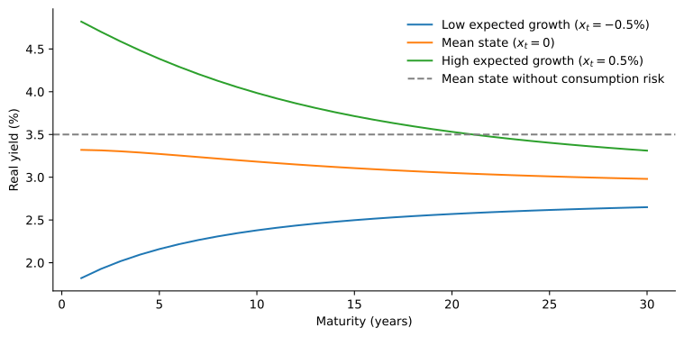
Figure 1 uses annual periods with \delta = 0.005, g = 1\%, \gamma = 3, \sigma_c = 2\%, \sigma_x = 0.5\% and \phi = 0.85. When expected growth is above its mean, short yields are high and the curve slopes down as growth is expected to return to normal. When it is below its mean, the curve slopes up. Without consumption risk the mean-state curve would be flat at \delta + \gamma g = 3.5\%. The precautionary term pulls every yield below that line, and pulls long yields down the most, so all three curves converge toward about 2.8\%. This is the downward slope of the example, now driven by persistence rather than by two hand-picked scenarios. Fixed-Income Securities in Discrete Time obtains state-dependent curves of the same kind from an affine model of the SDF.

A Dividend Claim, Horizon by Horizon

The same economy can price a stock. Let log dividend growth load on both consumption shocks and on expected growth, \Delta d_{t+1} = g_d + b_x\, x_t + b_c\,\sigma_c\,\varepsilon_{t+1} + \sigma_u\, u_{t+1}, where u_{t+1} is an independent standard normal shock specific to dividends. With b_c > 1, dividends are more exposed to consumption risk than consumption itself, as with a levered claim. Since \ln M_{t,t+j} and \ln D_{t+j} are jointly normal, each term of (8) factors as \operatorname{E}_t\!\left[M_{t,t+j} D_{t+j}\right] = Z_t^j\, \operatorname{E}_t(D_{t+j})\, e^{\omega_j}, \tag{14} where \omega_j is the conditional covariance between the logs of the SDF and the dividend, \omega_j = \operatorname{Cov}_t\!\left(\ln M_{t,t+j},\, \ln D_{t+j}\right) = -\gamma\Bigl(b_c\,\sigma_c^2\, j + b_x\,\sigma_x^2 \sum_{n=1}^{j-1} a_n^2\Bigr). \tag{15} The covariance term of (10) at horizon j is therefore Z_t^j\,\operatorname{E}_t(D_{t+j})(e^{\omega_j} - 1), and 1 - e^{\omega_j} is the fraction of the safe value of the j-th dividend lost to risk.⁶ Both pieces of \omega_j grow with the horizon. The first is short-run consumption risk accumulating period by period. The second is the long-run risk channel: a shock to expected growth moves consumption and dividends together for many periods, and its weight a_n^2 builds up with persistence.

⁶ The factorization uses \operatorname{E}(e^{Y}) = e^{\operatorname{E}(Y) + \operatorname{V}(Y)/2} for normal Y, applied to Y = \ln M_{t,t+j} + \ln D_{t+j}, whose variance is the two variances plus twice the covariance. The two variances reproduce Z_t^j and \operatorname{E}_t(D_{t+j}), leaving e^{\omega_j}. The covariance collects the shocks the two logs share: each \varepsilon contributes -\gamma \cdot b_c \sigma_c^2, and the shock \eta_{t+k} contributes -\gamma \cdot b_x \sigma_x^2 a_{j-k}^2, as in the footnote on cumulative growth.

Figure 2: Pricing a dividend claim horizon by horizon at the mean state x_t = 0, with D_t = 1. Top: the safe value Z^j\,\operatorname{E}(D_{t+j}) and the actual value \operatorname{E}[M_{t,t+j} D_{t+j}] of each dividend; the gap is the risk adjustment. Bottom: the share of the price that comes from dividends paid within j years.

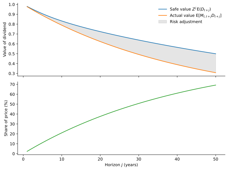
Figure 2 uses the parameters of Figure 1 with g_d = 1\%, b_c = b_x = 2.5 and \sigma_u = 5\%. The risk adjustment is negligible for the first dividend, 0.3\% of its safe value, but grows steadily with the horizon: 5\% at ten years, 23\% at thirty, and 39\% at fifty. Summed over all horizons, the price-dividend ratio is about 42, against 75 for the safe value of the same stream, so risk takes away almost half of the claim’s value, and over 90\% of that loss comes from dividends paid more than thirty years out. The bottom panel shows why those dividends matter: half of the price comes from dividends paid more than thirty years out. A stock is a long-duration asset, and its risk premium is earned mainly on the cash flows that are most exposed to long-run consumption risk. Risk Premia in Intertemporal Models prices this long-run channel in the framework of Bansal and Yaron (2004).⁷

⁷ This valuation side of long-run risk needs only power utility. Epstein-Zin preferences add the return side. Under power utility the one-period SDF does not load on the news shock \eta_{t+1}, so news about growth earns no premium when it arrives, and with \gamma > b_x the price-dividend ratio even falls on good news, since higher expected growth raises discount rates by more than it raises dividends. Epstein-Zin preferences price the news immediately, in proportion to \gamma - 1/\psi, and with \psi > 1 prices rise on good news, which is how Bansal and Yaron (2004) obtain a large equity premium with moderate risk aversion.

Bansal, Ravi, and Amir Yaron. 2004. “Risks for the Long Run: A Potential Resolution of Asset Pricing Puzzles.” Journal of Finance 59 (4): 1481–509.

Nominal Claims

Everything above is in units of consumption. Payoffs fixed in dollars are priced by converting them to consumption first. If \Pi_t is the price level, a dollar at t+j buys 1/\Pi_{t+j} units of consumption, whose value at t is M_{t,t+j}/\Pi_{t+j} units of consumption, or M_{t,t+j}\Pi_t/\Pi_{t+j} dollars. The nominal compounded SDF is therefore M_{t,t+j}^* = M_{t,t+j}\,\frac{\Pi_t}{\Pi_{t+j}}. A nominal zero-coupon bond paying one dollar at t+T has price Z_t^{*T} = \operatorname{E}_t[M_{t,t+T}^*], and a call option with strike K on a dollar-denominated asset price S_{t+T} has price \operatorname{E}_t[M_{t,t+T}^*(S_{t+T} - K)^+].⁸

⁸ Beyond the effect of expected inflation, nominal bonds are cheaper when inflation tends to be high in the states where consumption is scarce, since they then pay little in real terms exactly when payoffs are most valuable. This is the source of the inflation risk premium in nominal yields.

Where This Leads

The multiperiod pricing formula holds for any time-separable utility and any consumption process. What it leaves open is the compounded SDF itself, and the following notebooks fill it in from three directions. Intertemporal Portfolio Choice derives the SDF from the investor’s portfolio problem when investment opportunities change over time. Recursive Preferences in a Multiperiod Economy drops time separability and shows that the SDF then depends on the return on wealth as well as consumption growth. Lognormal Consumption Growth adds distributional assumptions that turn (8) into closed forms.⁹

⁹ The Lucas tree of that notebook is the infinite-horizon dividend stream of this notebook with dividends equal to consumption, and its condition \kappa < 1 is the transversality condition (7).