Fixed-Income Securities in Discrete Time
Bond pricing is one of the most natural applications of the stochastic discount factor framework. The SDF approach is particularly powerful here because it handles an entire term structure (bonds of all maturities) within a single, unified pricing equation. By specifying the SDF and the dynamics of a small number of state variables, we obtain closed-form or recursively computable prices for bonds of every maturity simultaneously, without having to model each maturity separately. The framework also cleanly separates the physical dynamics of interest rates from the risk-neutral dynamics that determine prices, making it transparent how risk premia shape the yield curve.
This notebook develops the theory in discrete time, starting from the basic pricing equation for zero-coupon bonds and working through three progressively richer term-structure models: the Vasicek (1977) model with constant risk premia, the Cox et al. (1985) model with conditionally heteroscedastic interest rates, and the essentially affine class of Duffee (2002). We conclude with an N-factor Gaussian model, which combines the multifactor affine framework of Duffie and Kan (1996) and Dai and Singleton (2000) with the essentially affine prices of risk of Duffee (2002). The same ideas extend naturally to continuous time, where Itô’s lemma turns the pricing recursions into ordinary differential equations for the bond-price coefficients. That treatment is taken up in the bond pricing in continuous time notebook.
Zero-Coupon Bonds
A zero-coupon bond with maturity n is a claim to one unit of the numeraire, say one dollar, paid with certainty at time t + n, with no intermediate cash flows. It is the simplest possible fixed-income security, and every coupon bond can be decomposed into a portfolio of zero-coupon bonds, so understanding their pricing is the foundation of the entire term structure.
Denote the price of the n-period zero-coupon bond at time t by P_{nt}. One period later the same bond has one fewer period to maturity and trades at P_{n-1,t+1}, which is random from the perspective of t. Applying the fundamental SDF pricing equation to this one-period payoff gives
P_{nt} = \operatorname{E}_{t}(M_{t+1} P_{n-1,t+1}). \tag{1}
This is a recursion: the n-period price is determined by the (n-1)-period price one period ahead, weighted by the SDF. The boundary condition is P_{0t} = 1 for all t: a bond that has already matured pays its face value of one. Iterating (1) forward from this boundary condition, and applying the law of iterated expectations, gives
P_{nt} = \operatorname{E}_{t}(M_{t+1} M_{t+2} \cdots M_{t+n}).
This expression is intuitive: the price of a multi-period bond is the expected value of all the discounting that will occur between now and maturity. A high SDF in any future period, indicating that wealth is scarce and marginal utility is high, will reduce the bond price, reflecting the opportunity cost of tying up resources.
It is convenient to work in logs throughout. Write p_{nt} = \log P_{nt} and m_{t+1} = \log M_{t+1}. If the vector (m_{t+1}, p_{n-1,t+1}) is conditionally normal, as will be the case in all the models below, then the pricing equation (1) becomes exact in log form:
p_{nt} = \operatorname{E}_{t}(m_{t+1} + p_{n-1,t+1}) + \frac{1}{2}\operatorname{V}_{t}(m_{t+1} + p_{n-1,t+1}).
The variance term arises from Jensen’s inequality: \operatorname{E}(e^X) = e^{\operatorname{E}(X) + \frac{1}{2}\operatorname{V}(X)} for a normal X. It is sometimes called the convexity correction: uncertainty about future prices raises the bond price relative to what a naive expectation would suggest, because the exponential function is convex.
The continuously compounded yield to maturity y_{nt} is defined by P_{nt} = e^{-n y_{nt}}, so y_{nt} = -p_{nt}/n. It is the constant per-period discount rate that reproduces the observed price. The one-period yield y_{1t} = -p_{1t} is simply the current risk-free rate. Long yields are weighted averages of expected future short rates, adjusted for risk premia and convexity. Unpacking this decomposition is the main goal of the term-structure models that follow.
An investor who buys the n-period bond at t and sells it one period later earns the log return r_{n,t+1} = p_{n-1,t+1} - p_{nt}. This return is uncertain because the resale price p_{n-1,t+1} depends on the short rate prevailing at t+1. The Jensen-corrected expected excess return over the risk-free rate is the log risk premium:
\operatorname{E}_{t} r_{n,t+1} - y_{1t} + \frac{1}{2}\operatorname{V}_{t} r_{n,t+1} = -\operatorname{Cov}_{t}(p_{n-1,t+1}, m_{t+1}).
This expression is the central result for bond risk premia. It says that the premium an investor earns from holding a long bond is determined entirely by the conditional covariance between the bond’s resale price and the log SDF. If this covariance is negative, meaning the bond price tends to fall exactly when the SDF is high (in recessions), then the bond is risky in the sense that matters to investors, and it must compensate them with a positive expected excess return. Conversely, if the bond price rises in bad times, it functions as insurance and investors are willing to accept a lower, even negative, excess return. Understanding what drives this covariance, and in particular whether it is constant or time-varying, is the key empirical question in term-structure modeling.
The Vasicek Model
Vasicek (1977) is the simplest term-structure model that fits inside the SDF framework. It has a single state variable x_t representing the short-term interest rate, which evolves as a stationary first-order autoregression:
x_{t+1} = \mu + \phi x_{t} + \sigma \varepsilon_{t+1}, \qquad \varepsilon_{t+1} \overset{\text{iid}}{\sim} \mathcal{N}(0,1).
The parameter \phi \in (0, 1) controls persistence, that is, how quickly the short rate reverts to its unconditional mean \mu/(1-\phi) after a shock. The parameter \sigma is the standard deviation of the innovation. Because \varepsilon_{t+1} is normal and the AR(1) is linear, x_{t+1} is conditionally normal given the current state, which will make all bond prices tractable.
The log SDF takes the form
m_{t+1} = -x_{t} - \frac{1}{2}\left(\frac{\lambda}{\sigma}\right)^{2} - \left(\frac{\lambda}{\sigma}\right)\varepsilon_{t+1},
where \lambda is a single constant, the market price of interest-rate risk. The SDF loads on the same shock \varepsilon_{t+1} that drives the short rate. When \lambda < 0, the loading -\lambda/\sigma is positive, so the SDF rises when \varepsilon_{t+1} is positive, that is, when rates rise unexpectedly. Long bonds lose value when rates rise (since B_{n-1} < 0), so they do poorly precisely when the SDF is high. Assets that lose value in high-SDF states carry systematic risk and must compensate investors with a positive risk premium. The calibration below uses \lambda < 0, consistent with the empirical evidence that long bonds earn positive excess returns on average.
The constant -\frac{1}{2}(\lambda/\sigma)^2 is a Jensen correction that keeps the model internally consistent: it ensures that M_{t+1} = e^{m_{t+1}} satisfies the correct normalization \operatorname{E}_t(M_{t+1} R^f_{t+1}) = 1 where R^f_{t+1} = e^{x_t} is the gross risk-free return.
To see this, note that conditional on \mathcal{F}_t, the log SDF is normally distributed:
m_{t+1} \sim \mathcal{N}\left(-x_t - \frac{1}{2}\left(\frac{\lambda}{\sigma}\right)^2,\; \left(\frac{\lambda}{\sigma}\right)^2\right).
Applying the log-linear pricing equation to a one-period bond, whose payoff is simply 1 so that p_{0,t+1} = 0, gives
p_{1t} = \operatorname{E}_{t}(m_{t+1}) + \frac{1}{2}\operatorname{V}_{t}(m_{t+1}) = -x_{t} - \frac{1}{2}\left(\frac{\lambda}{\sigma}\right)^{2} + \frac{1}{2}\left(\frac{\lambda}{\sigma}\right)^{2} = -x_{t}.
The Jensen correction from the variance exactly cancels the -\frac{1}{2}(\lambda/\sigma)^2 in the mean of m_{t+1}, leaving p_{1t} = -x_t and therefore y_{1t} = x_t. The state variable is the short rate, a convenient normalization that gives x_t a direct empirical interpretation.
Solving the Model
For n > 1, guess the affine form
p_{nt} = A_{n} + B_{n} x_{t}.
Substituting into the log-linear pricing equation and matching coefficients in x_t yields the Riccati recursions:
\begin{aligned} A_{n} &= A_{n-1} + B_{n-1}(\mu - \lambda) + \frac{1}{2} B_{n-1}^{2} \sigma^{2}, \\ B_{n} &= \phi B_{n-1} - 1, \end{aligned} \tag{2}
with A_0 = 0 and B_0 = 0. The B_n recursion is linear and solves to
B_{n} = -\frac{1 - \phi^{n}}{1 - \phi}.
When |\phi| < 1, B_n \to -1/(1-\phi) as n \to \infty: long-duration bonds have exposures to the short rate that saturate at a finite level. The A_n coefficients are then determined by iterating the first recursion forward from A_0 = 0.
Implications
The affine solution has two notable implications. To compute the risk premium, note that p_{n-1,t+1} = A_{n-1} + B_{n-1} x_{t+1} is linear in \varepsilon_{t+1} with loading B_{n-1}\sigma, while m_{t+1} loads on the same shock with coefficient -\lambda/\sigma. Their conditional covariance is therefore \operatorname{Cov}_t(p_{n-1,t+1}, m_{t+1}) = B_{n-1}\sigma \cdot (-\lambda/\sigma) = -B_{n-1}\lambda, and the log risk premium is
\operatorname{E}_{t} r_{n,t+1} - y_{1t} + \frac{1}{2}\operatorname{V}_{t} r_{n,t+1} = -\operatorname{Cov}_{t}(p_{n-1,t+1}, m_{t+1}) = B_{n-1}\lambda.
This is constant: it depends only on maturity n, not on the current state x_t. Because B_{n-1} is deterministic and \lambda is a fixed parameter, the risk premium every investor earns from rolling into an n-period bond is the same regardless of whether rates are high or low, rising or falling. All variation in the yield curve in Vasicek therefore reflects variation in expectations about future short rates, not time-varying risk premia. This is a clean and testable prediction, and it is strongly rejected in the data: Fama and Bliss (1987) show that forward rates track variation through time in one-year expected returns on Treasury bonds, so term premia are not constant.
The forward rate for the period (t+n, t+n+1), defined by f_{nt} = p_{nt} - p_{n+1,t}, is obtained by differencing the affine bond prices. Substituting the solution for A_n and B_n gives
f_{nt} = \frac{\mu - \lambda}{1 - \phi} - \left(\frac{1-\phi^n}{1-\phi}\right)^{2}\frac{\sigma^{2}}{2} + \phi^{n}\left(x_{t} - \frac{\mu-\lambda}{1-\phi}\right).
The forward curve has three components. The first term, (\mu-\lambda)/(1-\phi), is the risk-neutral long-run mean of the short rate, the level to which all forward rates converge at long horizons. The second term is the convexity correction, which is always negative and grows in magnitude with maturity, pulling long forward rates below the long-run mean. The third term captures the current position of the short rate relative to its long-run mean: if x_t is above (\mu-\lambda)/(1-\phi), the forward curve slopes downward; if x_t is below it, the curve slopes upward. The model can therefore generate upward-sloping, flat, inverted, or slightly humped curves, but only by varying the level of x_t, and the shape is otherwise tightly constrained by the single factor.
The Risk-Neutral Measure
The SDF changes the drift of the short rate from \mu to \mu - \lambda without altering the volatility, giving the risk-neutral dynamics x_{t+1} = (\mu - \lambda) + \phi x_{t} + \sigma \varepsilon^{*}_{t+1}. Under this measure bond prices satisfy P_{nt} = e^{-y_{1t}} \operatorname{E}^{*}_{t}(P_{n-1,t+1}), which yields exactly the same recursions (2). The N-factor section below works out the general change-of-measure argument in full.
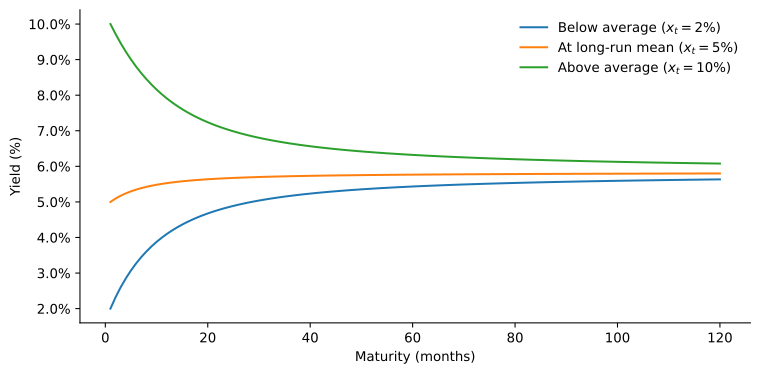
Figure 1 illustrates the model’s yield curve predictions under three scenarios for the current short rate x_t relative to its long-run mean of 5%. One period is a month, with persistence \phi = 0.97, and all rates are quoted at annual rates. When x_t = 2\%, rates are below their long-run mean and the market expects them to rise, producing an upward-sloping curve whose slope diminishes at long maturities as expectations converge to the steady state. When x_t = 5\%, the curve is nearly flat, with a slight upward tilt generated by the positive term premium B_{n-1}\lambda > 0. When x_t = 10\%, rates are above their long-run mean and expected to fall, inverting the curve. The Vasicek model thus captures the three most commonly observed yield curve shapes. What it cannot capture is any change in those shapes that is not driven purely by the level of x_t. Rich empirical patterns such as time-varying curvature or independently moving slope are inherently beyond a single-factor model.
The Cox-Ingersoll-Ross Model
Cox et al. (1985) derive the short rate from a general equilibrium model. Relative to Vasicek, its conditional variance is proportional to its level:
x_{t+1} = \mu + \phi x_{t} + \sigma x_{t}^{1/2} \varepsilon_{t+1}.
The log SDF is adjusted accordingly:
m_{t+1} = -x_{t} - \frac{1}{2}\left(\frac{\lambda}{\sigma}\right)^{2} x_{t} - \left(\frac{\lambda}{\sigma}\right) x_{t}^{1/2}\varepsilon_{t+1}.
Both the diffusion of the short rate and the market price of risk now scale with x_t^{1/2}, preserving the affine structure of log bond prices. Guessing p_{nt} = A_n + B_n x_t and matching coefficients yields:
\begin{aligned} A_{n} &= A_{n-1} + B_{n-1}\mu, \\ B_{n} &= -1 + (\phi - \lambda)B_{n-1} + \frac{1}{2}\sigma^{2}B_{n-1}^{2}, \end{aligned} \tag{3}
with A_0 = B_0 = 0. The B_n recursion is now quadratic (a Riccati equation) and generally must be iterated numerically.
The log risk premium in the CIR model is
\operatorname{E}_{t} r_{n,t+1} - y_{1t} + \frac{1}{2}\operatorname{V}_{t} r_{n,t+1} = B_{n-1}\lambda x_{t}.
Unlike Vasicek, the risk premium now inherits the time variation of x_t: when rates are high, bonds carry larger risk premia. This heteroscedastic structure is more consistent with the empirical finding that the slope of the yield curve forecasts bond excess returns. In continuous time the square-root diffusion keeps rates positive under the Feller condition, a property the Gaussian Vasicek model lacks. This discrete version does not inherit it: with normal \varepsilon_{t+1}, x_{t+1} is conditionally normal and can turn negative, after which x_{t+1}^{1/2} is undefined. The recursion (3) is best read as a discrete approximation to the continuous-time model, accurate when the period is short and x_t is far from zero.
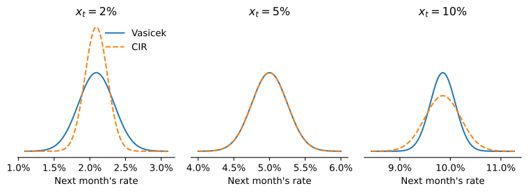
Figure 2 compares the conditional density of next month’s short rate in the two models, for the three values of x_t used in Figure 1. Both models share \mu and \phi, so the densities have the same mean, and the CIR volatility parameter is chosen so that both have a standard deviation of 25 bp at the long-run mean of 5%. Away from the mean they differ. The Vasicek density has the same width at every rate, while the CIR standard deviation is proportional to x_t^{1/2}: about 16 bp at 2% and 35 bp at 10%. This is the heteroscedasticity that makes the CIR risk premium B_{n-1}\lambda x_t rise with the level of rates, and the shrinking volatility near zero is what keeps the continuous-time process positive.
A One-Factor Essentially Affine Model
In completely affine models such as CIR, the market price of risk is proportional to the conditional volatility x_t^{1/2}, so compensation for risk is a multiple of its variance and risk premia can vary only if volatility does. Duffee (2002) proposes a broader essentially affine class in which the market price of risk is affine in the state, so compensation can vary independently of volatility. The class also allows heteroscedastic factors. Its simplest member keeps the homoscedastic short rate of Vasicek and sets:
m_{t+1} = -x_{t} - \frac{1}{2}\left(\frac{\lambda}{\sigma}\right)^{2} x_{t}^{2} - \left(\frac{\lambda}{\sigma}\right) x_{t}\varepsilon_{t+1}.
The market price of risk (\lambda/\sigma)x_t now scales with the level of the short rate, even though the short rate innovation \sigma\varepsilon_{t+1} does not. Matching coefficients gives:
\begin{aligned} A_{n} &= A_{n-1} + B_{n-1}\mu + \frac{1}{2}\sigma^{2}B_{n-1}^{2}, \\ B_{n} &= -1 + (\phi - \lambda)B_{n-1}, \end{aligned} \tag{4}
with A_0 = B_0 = 0. Note that B_n now satisfies a linear recursion (as in Vasicek, not quadratic as in CIR), so it can be solved explicitly:
B_n = -\frac{1 - (\phi - \lambda)^n}{1 - (\phi - \lambda)}.
The risk premium takes the same form as in CIR,
\operatorname{E}_{t} r_{n,t+1} - y_{1t} + \frac{1}{2}\operatorname{V}_{t} r_{n,t+1} = B_{n-1}\lambda x_{t},
but the mechanism is different. Here conditional return volatility B_{n-1}\sigma is constant (it does not depend on x_t), yet the risk premium still varies with the level of the short rate because the market price of risk (\lambda/\sigma)x_t does. This separation of volatility from risk premia is what Duffee (2002) finds useful in the data: completely affine models forecast future Treasury yields worse than a random walk, and the essentially affine extension improves the forecasts.
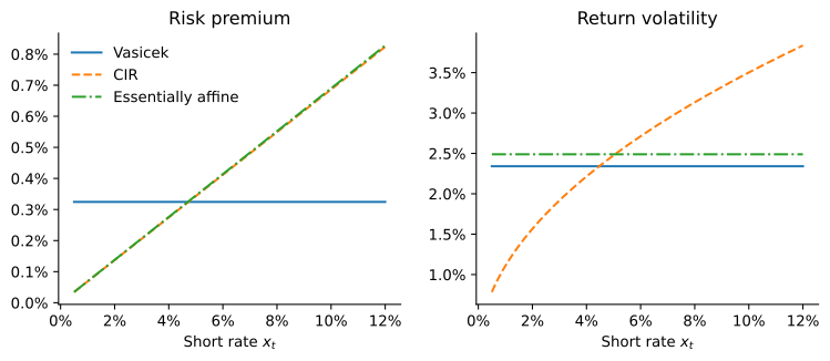
Figure 3 compares the three one-factor models for a ten-year zero-coupon bond held for one month. All three share \mu and \phi, CIR uses the volatility of Figure 2, and the CIR and essentially affine models set \lambda equal to the Vasicek value divided by the long-run mean of the short rate, so the three premia nearly coincide at x_t = 5\%. In Vasicek neither the premium nor the volatility moves with x_t. In CIR both rise, and the premium is proportional to the variance of the return, so high premia come only with high volatility. In the essentially affine model the premium rises with x_t as in CIR, while the volatility stays flat as in Vasicek.
An N-Factor Essentially Affine Model
The multifactor affine models of Duffie and Kan (1996) and Dai and Singleton (2000) replace the scalar short rate with a vector of state variables. This section takes the Gaussian case, the A_0(N) subfamily in the classification of Dai and Singleton (2000), with the essentially affine prices of risk of Duffee (2002). Let x_t \in \mathbb{R}^N follow the VAR:
x_{t+1} = \mu + \Phi x_{t} + \Sigma\varepsilon_{t+1},
where \mu \in \mathbb{R}^N, \Phi is an N \times N matrix, \Sigma is invertible, and \varepsilon_{t+1} \overset{\text{iid}}{\sim} \mathcal{N}(0, I_N). The log SDF is
\begin{aligned} m_{t+1} &= -(\delta_{0} + \delta_{1}' x_{t}) - \frac{1}{2}\Lambda_{t}'\Lambda_{t} - \Lambda_{t}'\varepsilon_{t+1}, \\ \Lambda_{t} &= \Sigma^{-1}(\lambda_{0} + \lambda_{1} x_{t}), \end{aligned}
where \delta_0 \in \mathbb{R}, \delta_1, \lambda_0 \in \mathbb{R}^N, and \lambda_1 is an N \times N matrix. The short rate is y_{1t} = \delta_0 + \delta_1' x_t. The essentially affine market price of risk \Lambda_t is affine in x_t, nesting the one-factor model as a special case.
Pricing the Bonds
Guessing the affine solution p_{nt} = A_n + B_n' x_t with B_n \in \mathbb{R}^N and applying the log-linear pricing equation gives:
\begin{aligned} A_{n} &= A_{n-1} + B_{n-1}'(\mu - \lambda_{0}) - \delta_{0} + \frac{1}{2}B_{n-1}'\Sigma\Sigma' B_{n-1}, \\ B_{n}' &= B_{n-1}'(\Phi - \lambda_{1}) - \delta_{1}', \end{aligned} \tag{5}
subject to A_0 = 0 and B_0 = 0. Comparing with the one-factor case, the risk adjustment replaces (\mu - \lambda) with (\mu - \lambda_0) and (\phi - \lambda) with (\Phi - \lambda_1): the market price of risk shifts the drift of the state vector under the risk-neutral measure.
Risk-Neutral Pricing
Under the risk-neutral measure, the state dynamics become:
x_{t+1} = (\mu - \lambda_{0}) + (\Phi - \lambda_{1}) x_{t} + \Sigma\varepsilon^{*}_{t+1},
and bond prices satisfy P_{nt} = e^{-y_{1t}}\operatorname{E}^{*}_t(P_{n-1,t+1}). The recursion (5) is the coefficient-matching consequence of this risk-neutral pricing equation. The physical parameters (\mu, \Phi) govern the time-series behavior of interest rates, while the risk-neutral parameters (\mu - \lambda_0, \Phi - \lambda_1) determine the cross-sectional shape of the yield curve. The essentially affine specification allows these to differ freely, which Duffee (2002) shows helps forecast yields. In this Gaussian setting, completely affine models are the special case \lambda_1 = 0. The Gaussian model is far from the most general affine model: state-dependent volatility and factors that stay positive fit the same recursive pricing structure once the state is specified through its conditional Laplace transform (Darolles et al. 2006; Le et al. 2010), but that extension is beyond the scope of these notes.
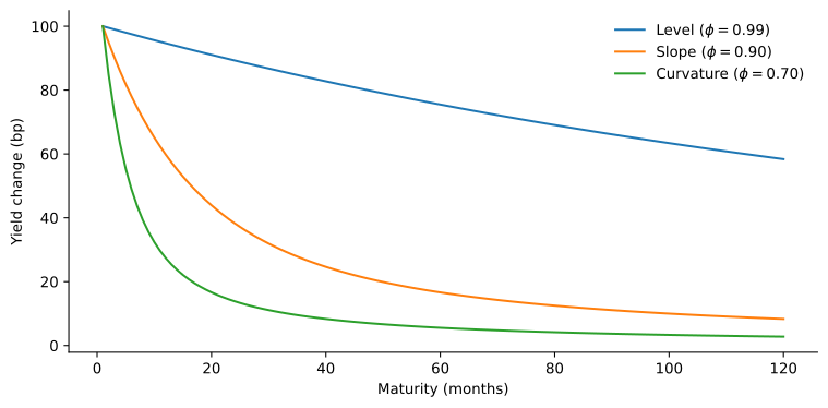
Figure 4 shows how each factor transmits a 100 bp shock to yields at different maturities. All three factors affect the short rate equally (each shock raises the one-month yield by 100 bp), but they differ sharply in how quickly that effect fades with maturity. The persistent factor (\phi = 0.99) moves even ten-year yields by roughly 60 bp, so it acts like a level factor. The intermediate factor (\phi = 0.90) mean-reverts faster, and its yield effect declines to about 8 bp by maturity 120, so a positive shock tilts the curve downward, as a slope factor would. The transitory factor (\phi = 0.70) mean-reverts fastest of all: the yield effect drops sharply in the first year and is negligible beyond five years, so it essentially only moves the shortest part of the curve.
None of the three produces curvature. With a diagonal \Phi, the loading of the n-period yield on factor k is \delta_{1k}(1-\phi_k^n)/\bigl(n(1-\phi_k)\bigr), which declines monotonically with maturity. A curvature factor needs a hump-shaped loading, which arises when \Phi is not diagonal, for example when one factor drives the expected change of another. Litterman and Scheinkman (1991) find that three factors, which they call level, steepness and curvature, explain at least 96\% of the variability of excess returns on zero-coupon Treasuries, and the multi-factor affine model provides an arbitrage-free foundation for that decomposition once \Phi is rich enough to deliver all three shapes.