Intertemporal Portfolio Choice
Introduction
The two-date problem of consumption and portfolio choice treats investment opportunities as fixed. In practice they change over time: interest rates fluctuate, risk premia vary with the business cycle, and volatility clusters. A long-horizon investor therefore cares not only about the return on the portfolio over the next period, but also about how that return relates to the opportunities that will be available afterward.
This notebook solves the consumption and portfolio problem over an infinite horizon when a vector of state variables z_t drives the investment opportunity set. The Bellman equation and the envelope condition deliver the SDF of Multiperiod Asset Pricing, now derived from the investor’s own problem and written in terms of the value function. A first-order approximation of the value function then turns the SDF into a linear factor model, with the return on wealth and the innovations in the state variables as factors. It delivers Merton’s intertemporal CAPM (Merton 1973) for risk premia, and an optimal portfolio made of a myopic demand and a hedging demand.
The Investment Problem
An investor with wealth W_t chooses consumption C_t and a vector \pmb{\alpha}_t of portfolio weights in N risky assets, with the rest of savings in a one-period risk-free asset, to maximize \operatorname{E}_t \sum_{i=0}^\infty \beta^i\, u(C_{t+i}) subject to the budget constraint W_{t+1} = R^w_{t+1}(W_t - C_t), \qquad R^w_{t+1} = R^f_{t+1} + \pmb{\alpha}_t'\mathbf{R}^{\,e}_{t+1}. \tag{1} Here \mathbf{R}_{t+1} is the vector of gross risky returns, R^f_{t+1} is the gross risk-free return, known at t, and \mathbf{R}^{\,e}_{t+1} = \mathbf{R}_{t+1} - R^f_{t+1}\pmb{\imath} is the vector of excess returns. Savings W_t - C_t are invested between t and t+1 and are the only resources available for future consumption.
The investment opportunity set is summarized by a vector of state variables z_t, such as dividend yields, term spreads, or volatility, that follows a Markov process. The conditional distribution of (\mathbf{R}_{t+1}, z_{t+1}) given z_t, and the risk-free rate R^f_{t+1}, depend on z_t. The joint distribution matters: innovations to z_{t+1} are in general correlated with returns, and that correlation is what lets an investor hedge changes in future opportunities by trading today. The investor’s situation at t is fully described by the pair (W_t, z_t), current resources and current opportunities.
Bellman Equation and Optimality Conditions
Let V(W_t, z_t) be the maximum expected utility attainable from (W_t, z_t). Because the problem from t+1 onward has the same form as the original, starting from (W_{t+1}, z_{t+1}), the value function satisfies the Bellman equation1 V(W_t, z_t) = \max_{C_t,\,\pmb{\alpha}_t}\Bigl\{u(C_t) + \beta\,\operatorname{E}_t\!\left[V(W_{t+1}, z_{t+1})\right]\Bigr\}, \tag{2} with W_{t+1} given by (1). The infinite-horizon problem becomes a sequence of identical one-period decisions.
1 Splitting the objective into u(C_t) and the sum from t+1 onward, the continuation problem is to maximize \operatorname{E}_t[\beta\,\operatorname{E}_{t+1}\sum_{i\ge 0}\beta^i u(C_{t+1+i})] over future policies. Those policies may depend on what is known at t+1, so the maximum can be taken state by state inside the outer expectation, and in each state it equals V(W_{t+1}, z_{t+1}). This is Bellman’s principle of optimality.
With \partial W_{t+1}/\partial C_t = -R^w_{t+1} and \partial W_{t+1}/\partial \pmb{\alpha}_t = (W_t - C_t)\mathbf{R}^{\,e}_{t+1}, the first-order conditions are u'(C_t) = \beta\,\operatorname{E}_t\!\left[V_W(W_{t+1}, z_{t+1})\, R^w_{t+1}\right], \qquad \operatorname{E}_t\!\left[V_W(W_{t+1}, z_{t+1})\,\mathbf{R}^{\,e}_{t+1}\right] = \mathbf{0}, \tag{3} where V_W = \partial V/\partial W is the marginal value of wealth, and the common factor \beta(W_t - C_t) > 0 has been divided out of the portfolio condition. The first condition says that the utility lost by consuming one unit less today equals the expected discounted value of the extra wealth carried into tomorrow. The second says that no reallocation toward any risky asset raises expected utility, once returns are weighted by the marginal value of wealth in each state.
Differentiating the Bellman equation with respect to W_t at the optimal policies gives the envelope condition2 V_W(W_t, z_t) = \beta\,\operatorname{E}_t\!\left[V_W(W_{t+1}, z_{t+1})\, R^w_{t+1}\right] = u'(C_t). \tag{4} At the optimum, an extra dollar of wealth is worth the same whether it is consumed today or invested, as in the two-date problem.
2 The derivative of the right-hand side of (2) contains terms in \partial C_t^*/\partial W_t and \partial \pmb{\alpha}_t^*/\partial W_t, how the optimal policies respond to wealth. The first is multiplied by u'(C_t) - \beta\operatorname{E}_t[V_W R^w_{t+1}] and the second by (W_t - C_t)\,\beta\operatorname{E}_t[V_W \mathbf{R}^{\,e}_{t+1}], both zero by (3). What remains is the direct effect, \beta\operatorname{E}_t[V_W R^w_{t+1}]. The argument is the same as in the two-date problem of consumption and portfolio choice.
The Stochastic Discount Factor
The envelope condition suggests the pricing kernel M_{t+1} = \beta\,\frac{V_W(W_{t+1}, z_{t+1})}{V_W(W_t, z_t)} = \beta\,\frac{u'(C_{t+1})}{u'(C_t)}. \tag{5} It prices every asset. The portfolio condition in (3) gives \operatorname{E}_t[M_{t+1}\mathbf{R}^{\,e}_{t+1}] = \mathbf{0}, and the envelope condition gives \operatorname{E}_t[M_{t+1}R^w_{t+1}] = 1. Since R^w_{t+1} = R^f_{t+1} + \pmb{\alpha}_t'\mathbf{R}^{\,e}_{t+1}, the second condition reduces to R^f_{t+1}\operatorname{E}_t(M_{t+1}) = 1, so M_{t+1} prices the risk-free asset, and then \operatorname{E}_t[M_{t+1}\mathbf{R}_{t+1}] = R^f_{t+1}\operatorname{E}_t(M_{t+1})\pmb{\imath} + \operatorname{E}_t[M_{t+1}\mathbf{R}^{\,e}_{t+1}] = \pmb{\imath}.
The second form in (5) is the consumption-based kernel of Multiperiod Asset Pricing and of the intertemporal asset-pricing literature (Lucas 1978; Breeden 1979). The first form is the one this notebook uses. It shows that the SDF moves with anything that moves the marginal value of wealth: shocks to wealth itself, and news about future investment opportunities through z_{t+1}.
A Linear Approximation
The value function is rarely known in closed form, but a first-order expansion of V_W around (W_t, z_t) is enough to see how the SDF depends on the two kinds of shocks:3 V_W(W_{t+1}, z_{t+1}) \approx V_W(W_t, z_t) + V_{WW}(W_t, z_t)(W_{t+1} - W_t) + V_{Wz}(W_t, z_t)'\,\Delta z_{t+1}, where \Delta z_{t+1} = z_{t+1} - z_t and V_{Wz} is the vector of cross derivatives. Dividing by V_W(W_t, z_t) brings in three quantities. Relative risk aversion of the value function, rra_t = -W_t V_{WW}/V_W, measures the curvature of indirect utility in wealth. The hedging coefficients h_t = -V_{Wz}/V_W measure how the marginal value of wealth responds to the state variables. The consumption-wealth ratio k_t = C_t/W_t enters through the budget constraint, since W_{t+1} = R^w_{t+1}(1-k_t)W_t and hence (W_{t+1} - W_t)/W_t = R^w_{t+1}(1-k_t) - 1. Substituting into (5), M_{t+1} \approx \beta\left[1 - rra_t\bigl(R^w_{t+1}(1-k_t) - 1\bigr) - h_t'\,\Delta z_{t+1}\right]. \tag{6}
3 The neglected terms are of second order in the changes over one period, so the approximation improves as the period shrinks. In continuous time, Itô’s lemma keeps exactly the terms that survive, and the corresponding expression for d\Lambda/\Lambda in Optimal Portfolio and Consumption in Continuous Time is exact.
The SDF is high when wealth falls, with weight rra_t, and when the state variables move in the direction that raises the marginal value of wealth, with weights h_t. If the opportunity set were constant, the second channel would disappear and the model would reduce to a single wealth factor. For any return R^i_{t+1}, (6) gives the covariance decomposition \operatorname{Cov}_t(M_{t+1}, R^i_{t+1}) = -\beta\left[rra_t(1-k_t)\,\operatorname{Cov}_t(R^w_{t+1}, R^i_{t+1}) + h_t'\,\operatorname{Cov}_t(\Delta z_{t+1}, R^i_{t+1})\right]. \tag{7}
The Intertemporal CAPM
The pricing condition \operatorname{E}_t[M_{t+1} R^{e,i}_{t+1}] = 0 can be written as \operatorname{E}_t(M_{t+1})\,\operatorname{E}_t(R^{e,i}_{t+1}) + \operatorname{Cov}_t(M_{t+1}, R^{e,i}_{t+1}) = 0. Since \operatorname{E}_t(M_{t+1}) = 1/R^f_{t+1} and R^f_{t+1} is known at t, so that \operatorname{Cov}_t(M_{t+1}, R^{e,i}_{t+1}) = \operatorname{Cov}_t(M_{t+1}, R^i_{t+1}), this gives \operatorname{E}_t\, R^{e,i}_{t+1} = -R^f_{t+1}\operatorname{Cov}_t(M_{t+1}, R^i_{t+1}), and (7) then implies \operatorname{E}_t\, R^{e,i}_{t+1} = \beta^{w,i}_t\,\lambda^w_t + \left(\beta^{z,i}_t\right)'\lambda^h_t, \tag{8} where the betas measure asset i’s exposure to each source of risk, \beta^{w,i}_t = \frac{\operatorname{Cov}_t(R^i_{t+1}, R^w_{t+1})}{\sigma^2_t(R^w_{t+1})}, \qquad \beta^{z,i}_t = \left[\operatorname{Cov}_t(\Delta z_{t+1})\right]^{-1}\operatorname{Cov}_t(\Delta z_{t+1}, R^i_{t+1}), and the risk prices reward each unit of exposure: \lambda^w_t = \beta\, R^f_{t+1}\, rra_t(1-k_t)\,\sigma^2_t(R^w_{t+1}), \qquad \lambda^h_t = \beta\, R^f_{t+1}\operatorname{Cov}_t(\Delta z_{t+1})\, h_t. With several state variables, \beta^{z,i}_t is the vector of coefficients from a multiple regression of R^i_{t+1} on \Delta z_{t+1}, and \operatorname{Cov}_t(\Delta z_{t+1}) is the covariance matrix of the state variable innovations.
Equation (8) holds for any single investor. For a representative investor, whose wealth is the market portfolio, it is Merton’s intertemporal CAPM in discrete time. The first beta is the covariance with the investor’s wealth portfolio, as in the static CAPM. The second is the covariance with news about investment opportunities. An asset that pays off when the marginal value of wealth rises, because opportunities have deteriorated, is a hedge, and investors accept a lower expected return to hold it. Campbell (1993) develops a discrete-time version that replaces the state variables by news about future market returns, the approach of Risk Premia in Intertemporal Models.
Optimal Portfolio
The same condition determines the portfolio. Let \pmb{\Sigma}_t = \operatorname{Cov}_t(\mathbf{R}_{t+1}) be the conditional covariance matrix of risky returns, \pmb{\mu}^e_t = \operatorname{E}_t(\mathbf{R}^{\,e}_{t+1}) the vector of expected excess returns, and \pmb{\Sigma}^{z,R}_t = \operatorname{Cov}_t(\Delta z_{t+1}, \mathbf{R}_{t+1}) the matrix of covariances between state innovations and returns, with one row per state variable and one column per asset. Since R^w_{t+1} = R^f_{t+1} + \pmb{\alpha}_t'\mathbf{R}^{\,e}_{t+1}, the vector of covariances of the risky returns with the wealth return is \operatorname{Cov}_t(\mathbf{R}_{t+1}, R^w_{t+1}) = \pmb{\Sigma}_t\pmb{\alpha}_t. Stacking (8) over all assets, \pmb{\mu}^e_t = \beta\, R^f_{t+1}\, rra_t(1-k_t)\,\pmb{\Sigma}_t \pmb{\alpha}_t + \beta\, R^f_{t+1}\, \pmb{\Sigma}^{z,R\prime}_t h_t, and solving for the portfolio weights, \pmb{\alpha}_t = \underbrace{\frac{1}{\beta\, R^f_{t+1}\, rra_t(1-k_t)}\pmb{\Sigma}_t^{-1}\pmb{\mu}^e_t}_{\text{myopic demand}} \; \underbrace{- \frac{1}{rra_t(1-k_t)}\pmb{\Sigma}_t^{-1}\pmb{\Sigma}^{z,R\prime}_t h_t}_{\text{hedging demand}}. \tag{9}
The myopic demand is the tangency portfolio scaled inversely by risk aversion. It is the portfolio a one-period investor would hold, and the only term that survives when the opportunity set is constant. The factor 1-k_t appears because the linearization measures the wealth shock per dollar of beginning-of-period wealth, while only the fraction 1-k_t is invested. The factor \beta\, R^f_{t+1} is close to one when expected changes in wealth and in the state variables are small, since taking expectations of (6) gives \operatorname{E}_t(M_{t+1}) = 1/R^f_{t+1}.
The hedging demand consists of positions taken not for their expected return but for their covariance with the state variables. The matrix \pmb{\Sigma}_t^{-1}\pmb{\Sigma}^{z,R\prime}_t holds the portfolios of risky assets that best track each state variable, and h_t sets how much of each the investor wants. Its sign depends on preferences. Suppose a higher z means better opportunities, such as higher expected returns. Under power utility with \gamma > 1, wealth is most valuable when opportunities are poor, so V_W falls with z and h_t > 0. The investor then holds more of the assets that pay off when z falls, which insure against a deterioration in opportunities. With \gamma < 1 the sign reverses. With log utility the value function has the form \ln W_t/(1-\beta) + f(z_t), so V_W does not depend on z and the hedging demand vanishes even when opportunities vary. In that case, and whenever the opportunity set is constant, every investor holds the same risky portfolio \pmb{\Sigma}_t^{-1}\pmb{\mu}^e_t in different proportions, the two-fund separation of the static model.
Equation (9) characterizes the optimal portfolio rather than solving for it. The coefficients rra_t and h_t are derivatives of the value function, which depends on the entire optimal policy, so the formula says how demand splits into its two motives but delivers numbers only once V is known. Optimal Portfolio and Consumption in a One-Factor Gaussian Model solves for the value function explicitly in continuous time, and Campbell and Viceira (1999) show that hedging demands can be large when expected stock returns are predictable.
Example 1 Consider two uncorrelated stocks with annual return variances 0.04 and 0.0625 and expected excess returns 0.048 and 0.08, so \pmb{\Sigma}_t = \operatorname{diag}(0.04,\ 0.0625) and \pmb{\mu}^e_t = (0.048,\ 0.08)'. There is one state variable, whose innovation has covariances \pmb{\Sigma}^{z,R}_t = (0.016,\ -0.015) with the two returns. The investor has rra_t = 2, consumes k_t = 4\% of wealth each year, and h_t = 1, so the marginal value of wealth falls when z rises. For simplicity set \beta\, R^f_{t+1} = 1.
The myopic demand is \frac{1}{2 \times 0.96}\begin{pmatrix} 0.048 / 0.04 \\ 0.08 / 0.0625 \end{pmatrix} = \begin{pmatrix} 0.625 \\ 0.667 \end{pmatrix}, and the hedging demand is -\frac{1}{2 \times 0.96}\begin{pmatrix} 0.016 / 0.04 \\ -0.015 / 0.0625 \end{pmatrix} = \begin{pmatrix} -0.208 \\ 0.125 \end{pmatrix}, so \pmb{\alpha}_t = (0.417,\ 0.792)'. The second stock pays off when z falls, which is when wealth is most valuable, so the investor holds more of it than the myopic demand. The first stock pays off when z rises and is held less.
These are the two stocks of the continuous-time portfolio example, where the same inputs give a myopic demand of (0.60,\ 0.64)', a hedging demand of (-0.20,\ 0.12)', and \pmb{\alpha}^* = (0.40,\ 0.76)'. Every component here is larger by the factor 1/(1-k_t) = 1/0.96. In discrete time the investor consumes 4\% of wealth before investing the rest, so the weights apply to savings, a base smaller than wealth by the factor 1-k_t. The exposure of total wealth to each return, (1-k_t)\pmb{\alpha}_t, is exactly the continuous-time \pmb{\alpha}^*. In continuous time consumption over an interval dt is negligible, the factor disappears, and the formula holds exactly rather than as a linear approximation.
The example fixes h_t = 1, but the same market looks different to investors with different hedging motives. Figure 1 repeats the calculation of Example 1 for values of h_t between -2 and 2, holding everything else fixed.
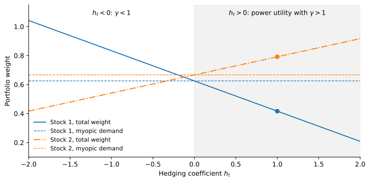
The myopic demands do not move: they depend only on expected returns, covariances and risk aversion. The hedging demand is linear in h_t, and because the two stocks covary with the state variable with opposite signs, the total weights fan out in opposite directions. An investor with h_t > 0, who values wealth most when z is low, tilts toward the second stock, which pays off in those states. An investor with h_t < 0 tilts the other way. The two investors face the same returns and agree on the myopic portfolio, yet hold different risky portfolios, because they disagree about which future states make wealth most valuable.
Where This Leads
The intertemporal CAPM in (8) rests on a linear approximation and on state variables that the theory does not name. The following notebooks address both. Recursive Preferences in a Multiperiod Economy shows that with Epstein-Zin preferences the return on wealth enters the SDF exactly, without approximating the value function. Risk Premia in Intertemporal Models then log-linearizes the budget constraint instead, which identifies the hedging factor as news about future market returns. In continuous time the same argument is exact, as Optimal Portfolio and Consumption in Continuous Time shows.