Lognormal Consumption Growth
This notebook develops the lognormal benchmark for asset pricing, starting with CRRA power utility and extending to Epstein-Zin recursive preferences. The lognormal setting is the workhorse framework for theoretical asset pricing because it yields closed-form expressions for the risk-free rate, the Hansen-Jagannathan bound, and log risk premia, all reducing to simple functions of means, variances, and covariances. This tractability follows from a single key property: when the log SDF and log returns are jointly normal, the pricing equation 1 = \operatorname{E}_t(M_{t+1} R^i_{t+1}) becomes an equation in moments rather than an integral. Risk premia then decompose into covariance terms with transparent economic interpretations, and comparative statics on preference parameters follow directly.
The lognormal framework is also the natural setting for diagnosing the two central puzzles in consumption-based asset pricing. Under CRRA preferences, matching the observed equity premium requires implausibly high risk aversion (Mehra and Prescott 1985), which in turn implies a counterfactually high risk-free rate (Weil 1989). The second puzzle arises because a single parameter governs both risk aversion and intertemporal substitution. Epstein-Zin preferences (Epstein and Zin 1989) decouple the two within the same lognormal environment, which resolves the risk-free rate puzzle. With i.i.d. consumption growth they leave the equity premium puzzle intact, since risk premia still require implausibly high risk aversion (Weil 1989). This tractability also underpins the asset pricing results developed in Risk Premia in Intertemporal Models, where the lognormal pricing equations derived here serve as the point of departure for the Campbell and Bansal-Yaron frameworks.
Let lowercase letters denote logs, so c_t = \ln(C_t) and \Delta c_{t+1} = c_{t+1} - c_t. Throughout, assume consumption growth is conditionally normal: \Delta c_{t+1} \sim \mathcal{N}\left(\operatorname{E}_t(\Delta c_{t+1}), \sigma_t^2(\Delta c_{t+1})\right). This assumption, together with joint normality of log returns and the log SDF, underlies all closed-form results derived below.
Power Utility
As a benchmark before introducing Epstein-Zin recursion, start with the standard power-utility model. This baseline pins down how interest rates and risk premia relate to marginal utility when risk aversion and intertemporal substitution are tied together. Preferences are CRRA (power utility): u(C) = \begin{cases} \frac{C^{1-\gamma}}{1-\gamma}, & \text{if}\ \gamma \geq 0, \gamma \neq 1 \\ \ln(C), & \text{if}\ \gamma = 1 \end{cases} with marginal utility u'(C) = C^{-\gamma}.
With \delta = -\ln(\beta), the log SDF is m_{t+1} = -\delta - \gamma \Delta c_{t+1}. Since m_{t+1} is an affine function of the conditionally normal \Delta c_{t+1}, it is also conditionally normal with \begin{aligned} \operatorname{E}_{t}(m_{t+1}) & = -\delta - \gamma \operatorname{E}_{t}(\Delta c_{t+1}), \\ \sigma^{2}_{t}(m_{t+1}) & = \gamma^{2} \sigma_{t}^{2}(\Delta c_{t+1}). \end{aligned}
The Risk-Free Rate
Since M_{t+1} = e^{m_{t+1}} is lognormal, applying the lognormal expectation formula gives \begin{aligned} \operatorname{E}_{t}(M_{t+1}) & = \exp\left( \operatorname{E}_{t}(m_{t+1}) + \frac{1}{2} \sigma^{2}_{t}(m_{t+1}) \right) \\ & = \exp\left( -\delta - \gamma \operatorname{E}_{t}(\Delta c_{t+1}) + \frac{1}{2} \gamma^{2} \sigma_{t}^{2}(\Delta c_{t+1}) \right). \end{aligned} Using r^f_{t+1} = -\ln \operatorname{E}_t(M_{t+1}), the log risk-free rate is r^f_{t+1} = \delta + \gamma \operatorname{E}_{t}(\Delta c_{t+1}) - \frac{1}{2} \gamma^{2} \sigma_{t}^{2}(\Delta c_{t+1}).
This expression implies three comparative statics for the real risk-free rate. Higher impatience (\delta) raises the risk-free rate. Higher expected consumption growth also raises the risk-free rate because if households expect to be richer tomorrow, they save less today, lowering bond demand and raising yields. By contrast, higher consumption-growth uncertainty lowers the risk-free rate through precautionary saving. In the data, the real risk-free rate is low and stable despite positive expected consumption growth. This tension, sometimes called the risk-free rate puzzle, is one that Epstein-Zin preferences help address by decoupling the precautionary-saving response from risk aversion.
A Lucas Tree with i.i.d. Growth
The simplest equilibrium application is an exchange economy with a single Lucas tree (Lucas 1978). The tree produces a perishable dividend that is the economy’s only source of consumption, so in equilibrium the dividend equals aggregate consumption, D_t = C_t. Suppose log consumption growth is i.i.d. normal, \Delta c_{t+1} \sim \mathcal{N}(g, \sigma_c^2). By the multiperiod pricing formula, the ex-dividend price of the tree is P_t = \operatorname{E}_t \sum_{j=1}^{\infty} \beta^j \left(\frac{C_{t+j}}{C_t}\right)^{-\gamma} C_{t+j} = C_t \sum_{j=1}^{\infty} \beta^j\, \operatorname{E}_t\!\left[\left(\frac{C_{t+j}}{C_t}\right)^{1-\gamma}\right]. Since \ln(C_{t+j}/C_t) is normal with mean jg and variance j\sigma_c^2, each expectation equals \exp\bigl(j\bigl[(1-\gamma)g + \frac{1}{2}(1-\gamma)^2\sigma_c^2\bigr]\bigr), and the sum is geometric.
Property 1 (Lucas Tree with i.i.d. Growth) Let \kappa = \exp\!\left(-\delta + (1-\gamma)g + \frac{1}{2}(1-\gamma)^2\sigma_c^2\right). If \kappa < 1, the price-dividend ratio of the tree is constant, \frac{P_t}{C_t} = \frac{\kappa}{1-\kappa}, \tag{3} and the log return on the tree is r_{t+1} = \Delta c_{t+1} - \ln\kappa. \tag{4}
The return follows from R_{t+1} = (P_{t+1} + C_{t+1})/P_t = (C_{t+1}/C_t)(1 + P/C)/(P/C) = (C_{t+1}/C_t)/\kappa. Because the price-dividend ratio is constant, the tree’s return moves one-for-one with consumption growth: its volatility is \sigma_c and V_{ic} = \sigma_c^2. Equation (2) then gives a log equity premium of \operatorname{E}(r_{t+1}) - r^f_{t+1} + \sigma_c^2/2 = \gamma\sigma_c^2. This can be checked directly: (4) gives \operatorname{E}(r_{t+1}) = \delta + \gamma g - \frac{1}{2}(1-\gamma)^2\sigma_c^2, and subtracting the risk-free rate \delta + \gamma g - \frac{1}{2}\gamma^2\sigma_c^2 leaves (\gamma - \frac{1}{2})\sigma_c^2.
Two further features of the solution are worth noting. First, \ln\kappa moves with expected growth at rate 1-\gamma. With log utility, \kappa = \beta and P/C = \beta/(1-\beta) whatever the growth rate. For \gamma > 1, higher expected growth lowers the price-dividend ratio: cash flows grow faster, but the risk-free rate rises by \gamma per unit of growth, because the elasticity of intertemporal substitution 1/\gamma is below one. Second, the tree is perfectly correlated with consumption, and hence with the SDF, so its Sharpe ratio is close to the Hansen-Jagannathan bound \gamma\sigma_c.
Example 2 Let \delta = 0.01, g = 0.02, \sigma_c = 0.01 and \gamma = 2, at annual frequency. Then \ln\kappa = -0.01 - 0.02 + \tfrac{1}{2}(0.0001) = -0.02995, \qquad \kappa = 0.9705, so P/C = 0.9705/0.0295 \approx 32.9. The risk-free rate is r^f = 0.01 + 2 \times 0.02 - \tfrac{1}{2}(4)(0.0001) = 4.98\%, the tree’s volatility is 1\%, and its log equity premium, \operatorname{E}(r) - r^f + \sigma_c^2/2, is \gamma\sigma_c^2 = 0.02\%.
These are the numbers of the continuous-time Lucas tree, which has the same risk-free rate and equity premium and a price-dividend ratio of 1/0.02995 \approx 33.4. The gap of about half a year’s dividend is a matter of timing: the discrete tree pays each year’s dividend at the end of the year, on average half a year later than the continuous flow. More generally, over a period of length \Delta t, 1 - \kappa \approx q\,\Delta t with q = \delta - (1-\gamma)g - \frac{1}{2}(1-\gamma)^2\sigma_c^2, the continuous-time dividend yield. If C denotes the consumption rate per unit of time, the dividend per period is C\,\Delta t, and the discrete price converges to C/q. Both versions fail in the same way: an equity premium of 0.02\% and a stock market as smooth as consumption, the equity premium puzzle discussed above.
Epstein-Zin Preferences
The standard CRRA time-additive model is equivalent to a recursive specification: the continuation value U_t satisfies the Bellman equation U_{t}^{1-\gamma} = (1-\beta) C_{t}^{1-\gamma} + \beta \operatorname{E}_{t} (U_{t+1}^{1-\gamma}). In this formulation, the agent’s attitude toward risk and their willingness to substitute consumption over time are both governed by the single parameter \gamma. Specifically, \gamma is the coefficient of relative risk aversion, while the elasticity of intertemporal substitution (EIS) is constrained to equal 1/\gamma. This tight link is a restrictive feature of the standard model: an agent who is very risk averse (large \gamma) is also forced to have a very low willingness to substitute consumption over time, even though these are conceptually distinct aspects of preferences.
The Epstein-Zin model (Epstein and Zin 1989) decouples these two parameters by introducing an additional scaling parameter \theta into the recursion: U_{t}^{\frac{1-\gamma}{\theta}} = (1-\beta) C_{t}^{\frac{1-\gamma}{\theta}} + \beta \left(\operatorname{E}_{t} (U_{t+1}^{1-\gamma})\right)^{\frac{1}{\theta}}, where \theta = \frac{1-\gamma}{1-1/\psi}. The parameter \psi now independently controls the EIS, so \gamma and \psi can be chosen freely to match empirical estimates of risk aversion and intertemporal substitution separately. When \psi = 1/\gamma we have \theta = 1 and the standard power utility model is recovered as a special case. Intuitively, \theta governs the relative weight on intertemporal substitution versus market-return news in the SDF: when \theta < 1 (equivalently, \gamma > 1/\psi for \psi > 1) the agent prefers early resolution of uncertainty, and this tilts the SDF toward the market-return factor.
The Budget Constraint
As established in Recursive Preferences in a Multiperiod Economy, wealth evolves according to W_{t+1} = R^w_{t+1} (W_{t} - C_{t}) \tag{5} where R^w_{t+1} is the gross return on the market portfolio, a claim to the agent’s entire future consumption stream.
The Stochastic Discount Factor
As derived in Recursive Preferences in a Multiperiod Economy, the stochastic discount factor takes the form M_{t+1} = \left[\beta \left(\frac{C_{t+1}}{C_{t}}\right)^{-\frac{1}{\psi}}\right]^{\theta}\left[\frac{1}{R^w_{t+1}}\right]^{1-\theta}. This expression makes the separation of preferences transparent. The first factor is an intertemporal substitution term: it depends on consumption growth raised to -1/\psi, the inverse of the EIS. The second factor captures the return on the market portfolio and reflects how utility is affected by revisions in future investment opportunities. In the standard power utility case (\theta = 1), the second factor vanishes and only consumption growth determines the SDF.
Taking logs, with \delta = -\ln \beta and lowercase letters denoting logs of their uppercase counterparts, the log SDF is m_{t+1} = - \theta \delta - (\theta/\psi) \Delta c_{t+1} - (1-\theta) r^w_{t+1}.
The Risk-Free Rate
Applying (1) to the risk-free asset gives r^f_{t+1} = -\operatorname{E}_t(m_{t+1}) - \frac{1}{2}\sigma^2_t(m_{t+1}), so r^f_{t+1} = \theta\delta + \frac{\theta}{\psi}\operatorname{E}_{t}(\Delta c_{t+1}) + (1-\theta)\operatorname{E}_{t}(r^w_{t+1}) - \frac{1}{2}\sigma^{2}_{t}(m_{t+1}), where \sigma^{2}_{t}(m_{t+1}) = (\theta/\psi)^{2}V_{cc,t} + (1-\theta)^{2}V_{ww,t} + 2(\theta/\psi)(1-\theta)V_{cw,t}, with V_{ww,t} = \sigma^{2}_{t}(r^w_{t+1}) and V_{cw,t} = \operatorname{Cov}_{t}(\Delta c_{t+1}, r^w_{t+1}). Setting \theta = 1 and \psi = 1/\gamma recovers the CRRA expression.
The decoupling is immediate: expected consumption growth enters with coefficient \theta/\psi and the precautionary saving term scales with (\theta/\psi)^2, both of which depend on \psi independently of \gamma. A high \gamma can therefore match the equity premium without mechanically inflating the risk-free rate, resolving the tension identified in the Power Utility section.
Log Risk Premium
Using (1) and substituting the EZ log SDF into -\operatorname{Cov}_t(m_{t+1}, r^i_{t+1}), the log risk premium for any asset i satisfies where V_{ic,t} = \operatorname{Cov}_{t}(r^i_{t+1}, \Delta c_{t+1}) and V_{iw,t} = \operatorname{Cov}_{t}(r^i_{t+1}, r^w_{t+1}). The left-hand side is the expected excess log return plus a convexity correction. The right-hand side loads on two covariances, with consumption growth and with the market return, with weights that depend on \theta and hence on the preference parameters \gamma and \psi.
When \psi = 1/\gamma we have \theta = 1, so \theta/\psi = \gamma and 1 - \theta = 0. Equation (6) then reduces to (2): risk is priced solely through consumption covariance at rate \gamma, and the market return plays no role.
Outside this special case, and when investment opportunities vary over time, the model is an intertemporal CAPM with two priced betas. The first, V_{ic,t}, captures short-run consumption risk, the same margin as CRRA. The second, V_{iw,t}, captures exposure to the market portfolio and reflects intertemporal hedging demand. Its weight 1 - \theta depends on how far preferences deviate from CRRA. In the empirically relevant case \gamma > 1 and \psi > 1, we have \theta < 0 and hence 1 - \theta > 1, so market-return covariance is priced more heavily than under CRRA. Such an agent also prefers early resolution of uncertainty, since \gamma > 1/\psi. Preference for early resolution alone is not enough: with \psi > 1 and 1/\psi < \gamma < 1 the agent still prefers early resolution, but 0 < \theta < 1. An asset that co-moves strongly with the market amplifies wealth fluctuations precisely when continuation utility is sensitive to them, making it riskier than its consumption beta alone would suggest.
With i.i.d. returns the two betas coincide. The consumption-wealth ratio is then a constant k, so \Delta c_{t+1} = r^w_{t+1} + \ln(1-k) and V_{ic,t} = V_{iw,t}. The right-hand side of (6) becomes (\theta/\psi + 1 - \theta)\,V_{iw,t} = \gamma V_{iw,t}, since \theta(1-1/\psi) = 1-\gamma. Risk premia are those of a CRRA investor with risk aversion \gamma, and \psi affects only the risk-free rate, as shown in Recursive Preferences in a Multiperiod Economy.
The risk-free rate then takes a simple form. Write g = \operatorname{E}(\Delta c_{t+1}) and \sigma_c = \sigma(\Delta c_{t+1}). With i.i.d. returns the SDF is M_{t+1} = \beta^\theta(1-k)^{1-\theta}(C_{t+1}/C_t)^{-\gamma}, and the wealth portfolio has gross return (C_{t+1}/C_t)/(1-k). Pricing it, \operatorname{E}(M_{t+1}R^w_{t+1}) = 1, pins down \ln(1-k) = -\delta + \frac{1}{\theta}\bigl[(1-\gamma)g + \frac{1}{2}(1-\gamma)^2\sigma_c^2\bigr]. Substituting into r^f = -\ln\operatorname{E}(M_{t+1}) and using (1-\theta)(1-\gamma)/\theta = \gamma - 1/\psi gives r^f = \delta + \frac{g}{\psi} - \frac{1}{2}\left(\gamma + \frac{\gamma - 1}{\psi}\right)\sigma_c^2. \tag{7} With \psi = 1/\gamma this is the CRRA rate \delta + \gamma g - \frac{1}{2}\gamma^2\sigma_c^2. Expected growth now enters with coefficient 1/\psi instead of \gamma.
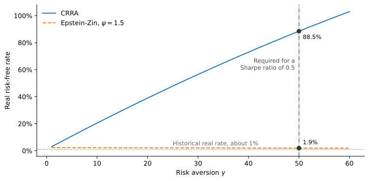
Example 3 Keep the parameters of Example 1 with \gamma = 50, and set \psi = 1.5. Then r^f = 0.01 + \frac{0.02}{1.5} - \tfrac{1}{2}\left(50 + \frac{49}{1.5}\right)(0.0001) \approx 1.9\%, against 88.5\% under CRRA.
The continuous-time equilibrium gives the same formula once its arithmetic growth rate \mu_c is written as g + \frac{1}{2}\sigma_c^2, and the same 1.9\%. Epstein-Zin preferences therefore resolve the risk-free rate puzzle. They do not resolve the equity premium puzzle with i.i.d. growth, since risk premia are those of CRRA and a Sharpe ratio of 0.5 still requires \gamma = 50. That takes persistent variation in expected growth, the subject of Risk Premia in Intertemporal Models.
Figure 1 puts the two examples side by side. Under CRRA the risk-free rate rises with \gamma because expected growth enters with coefficient \gamma, and by \gamma = 50 it is far above any historical real rate. Under Epstein-Zin expected growth enters with coefficient 1/\psi, and the rate stays near 2\% for every \gamma in the figure. The vertical line does not move, though: a Sharpe ratio of 0.5 needs \gamma = 50 under both preferences.