Generating Functions
Most of the random variables in this course are built by adding up simpler ones. The position of a random walk is a sum of coin flips, the number of defaults in a loan portfolio is a sum of default indicators, and the log return of a stock over a year is a sum of daily log returns. Computing the distribution of a sum directly is tedious, since it requires adding up the probabilities of all the ways in which the terms can combine. A generating function turns this problem into a much simpler one: it encodes the whole distribution of a random variable into a single function, and it converts sums of independent random variables into products of functions.
In these notes we study three closely related transforms. The probability generating function (PGF) is the natural tool for random variables that count things, like the number of heads, the number of defaults, or the number of steps until a random walk stops. The moment generating function (MGF) extends the idea to random variables with continuous values, such as normal returns. The characteristic function (CF) is the version that always exists, and it is the one used to prove limit theorems. All three are expectations of a function of the form e^{\theta X}, evaluated at different kinds of arguments.
Generating functions will reappear throughout the course. They provide the characteristic equation that solves the ruin problem, the exponential martingales used to study stopping times, the limit that turns rare Bernoulli events into a Poisson process, and the limit that turns a scaled random walk into a Brownian motion. For more complete treatments, see Blitzstein and Hwang (2019) and Grimmett and Stirzaker (2001). Feller (1968) remains the classic reference on generating functions for integer-valued random variables.
Probability Generating Functions
Definition
Let X be a random variable taking values in the natural numbers \mathbb{N} = \{0, 1, 2, \ldots\}, with probability mass function p_{X}(k) = \operatorname{P}(X = k). The probability generating function of X is G_{X}(z) = \operatorname{E}(z^{X}) = \sum_{k = 0}^{\infty} p_{X}(k) z^{k}. \tag{1} The PGF is a power series whose coefficients are the probabilities of X. Since the probabilities add up to one, the series converges at least for |z| \leq 1, and we always have G_{X}(1) = 1.
The variable z has no meaning of its own. It is a placeholder that keeps the probabilities in order: the coefficient of z^{k} is the probability that X = k. Because a power series determines its coefficients, we can recover the probability mass function from the PGF by differentiating at z = 0, p_{X}(k) = \frac{G_{X}^{(k)}(0)}{k!}, where G_{X}^{(k)} denotes the k-th derivative of G_{X}. Therefore, two random variables with the same PGF have the same distribution. This uniqueness property is what makes generating functions useful: if we can compute the PGF of a random variable and recognize it, we know its distribution.
Example 1 A Bernoulli random variable X takes the value 1 with probability p and the value 0 with probability 1 - p. It is the indicator of a single event, such as a coin landing heads or a borrower defaulting within a year. Its PGF is G_{X}(z) = (1 - p) z^{0} + p z^{1} = 1 - p + p z.
Example 2 Suppose we flip a coin that lands heads with probability p until we see the first head, and let X be the number of flips required. The first head occurs on flip k if the first k - 1 flips are tails and flip k is a head, so that p_{X}(k) = (1 - p)^{k - 1} p, \qquad k = 1, 2, 3, \ldots We say that X has a geometric distribution. Writing q = 1 - p, its PGF is a geometric series, G_{X}(z) = \sum_{k = 1}^{\infty} q^{k - 1} p z^{k} = p z \sum_{j = 0}^{\infty} (q z)^{j} = \frac{p z}{1 - q z}, which converges for |z| < 1 / q.
The geometric distribution is the simplest model of a waiting time in discrete time. Its continuous-time counterpart is the exponential distribution from the notes on continuous distributions, which describes the time between arrivals of a Poisson process.
Example 3 A random variable N has a Poisson distribution with parameter \lambda > 0 if p_{N}(k) = e^{-\lambda} \frac{\lambda^{k}}{k!}, \qquad k = 0, 1, 2, \ldots We write N \sim \text{Poisson}(\lambda). Using the power series e^{x} = \sum_{k = 0}^{\infty} x^{k} / k!, the PGF of N is G_{N}(z) = \sum_{k = 0}^{\infty} e^{-\lambda} \frac{\lambda^{k}}{k!} z^{k} = e^{-\lambda} \sum_{k = 0}^{\infty} \frac{(\lambda z)^{k}}{k!} = e^{-\lambda} e^{\lambda z} = e^{\lambda (z - 1)}.
The Poisson distribution counts the number of rare events that occur over a period of time, such as defaults in a large portfolio of loans, claims arriving at an insurance company, or large price jumps in a stock. We will see below why it arises so often.
Moments
The PGF also encodes the moments of X. Differentiating (1) term by term gives G_{X}'(z) = \sum_{k = 1}^{\infty} k \, p_{X}(k) z^{k - 1}, \qquad G_{X}''(z) = \sum_{k = 2}^{\infty} k (k - 1) \, p_{X}(k) z^{k - 2}. Setting z = 1 in each expression we obtain the factorial moments of X.
Proof
The first two expressions follow from setting z = 1 in the derivatives above, since G_{X}'(1) = \sum_{k} k \, p_{X}(k) = \operatorname{E}(X), \qquad G_{X}''(1) = \sum_{k} k (k - 1) \, p_{X}(k) = \operatorname{E}(X (X - 1)). For the variance, note that \operatorname{E}(X^{2}) = \operatorname{E}(X (X - 1)) + \operatorname{E}(X), so that \operatorname{V}(X) = \operatorname{E}(X^{2}) - \operatorname{E}(X)^{2} = G_{X}''(1) + G_{X}'(1) - G_{X}'(1)^{2}.Example 4 If N \sim \text{Poisson}(\lambda), then G_{N}(z) = e^{\lambda (z - 1)}, so that G_{N}'(z) = \lambda e^{\lambda (z - 1)} and G_{N}''(z) = \lambda^{2} e^{\lambda (z - 1)}. Therefore, \operatorname{E}(N) = \lambda, \qquad \operatorname{V}(N) = \lambda^{2} + \lambda - \lambda^{2} = \lambda. The mean and the variance of a Poisson random variable are both equal to \lambda.
Example 5 If X has the geometric distribution of Example 2, then G_{X}'(z) = \frac{p}{(1 - q z)^{2}}, \qquad G_{X}''(z) = \frac{2 p q}{(1 - q z)^{3}}. Evaluating at z = 1 and using 1 - q = p we find G_{X}'(1) = 1 / p and G_{X}''(1) = 2 q / p^{2}. Hence, \operatorname{E}(X) = \frac{1}{p}, \qquad \operatorname{V}(X) = \frac{2 q}{p^{2}} + \frac{1}{p} - \frac{1}{p^{2}} = \frac{q}{p^{2}}. For example, a die shows a six with probability p = 1/6, so we expect to wait 6 rolls for the first six.
Sums of Independent Random Variables
The most important property of generating functions is how they handle sums. If X and Y are independent, then z^{X} and z^{Y} are also independent, and, as shown in the notes on conditioning and independence, the expectation of a product of independent random variables is the product of their expectations.
Proof
Since z^{X + Y} = z^{X} z^{Y} and the random variables z^{X} and z^{Y} are independent, G_{X + Y}(z) = \operatorname{E}(z^{X} z^{Y}) = \operatorname{E}(z^{X}) \operatorname{E}(z^{Y}) = G_{X}(z) \, G_{Y}(z). The general case follows by applying this result repeatedly.Compare this with the direct approach. The probability that X + Y = k is \operatorname{P}(X + Y = k) = \sum_{j = 0}^{k} p_{X}(j) \, p_{Y}(k - j), a sum over all the ways of splitting k between X and Y. The PGF performs all these sums at once: multiplying two power series collects exactly these terms in the coefficient of z^{k}.
Example 6 Suppose a bank holds n loans, each defaulting independently with probability p. Let X_{i} be the Bernoulli indicator that loan i defaults, and let N = X_{1} + \cdots + X_{n} be the number of defaults. By Example 1 each X_{i} has PGF 1 - p + p z, so that G_{N}(z) = (1 - p + p z)^{n}. Expanding with the binomial theorem, G_{N}(z) = \sum_{k = 0}^{n} \binom{n}{k} p^{k} (1 - p)^{n - k} z^{k}, and reading off the coefficient of z^{k} gives the binomial distribution, \operatorname{P}(N = k) = \binom{n}{k} p^{k} (1 - p)^{n - k}. The moments follow just as easily: G_{N}'(1) = n p and G_{N}''(1) = n (n - 1) p^{2}, so that \operatorname{E}(N) = n p and \operatorname{V}(N) = n p (1 - p).
Example 7 If N_{1} \sim \text{Poisson}(\lambda_{1}) and N_{2} \sim \text{Poisson}(\lambda_{2}) are independent, then G_{N_{1} + N_{2}}(z) = e^{\lambda_{1} (z - 1)} e^{\lambda_{2} (z - 1)} = e^{(\lambda_{1} + \lambda_{2}) (z - 1)}, which is the PGF of a Poisson random variable with parameter \lambda_{1} + \lambda_{2}. By uniqueness, N_{1} + N_{2} \sim \text{Poisson}(\lambda_{1} + \lambda_{2}). If defaults in two independent sectors arrive as Poisson counts, total defaults are also a Poisson count.
Random Sums
In many applications the number of terms in a sum is itself random. An insurance company does not know in advance how many claims it will receive, and a market maker does not know how many orders will arrive during the next minute. Let N be a random variable taking values in \mathbb{N}, and let X_{1}, X_{2}, \ldots be independent and identically distributed random variables that are also independent of N. The random sum S = X_{1} + X_{2} + \cdots + X_{N} adds up a random number of terms, with the convention that S = 0 when N = 0. Its PGF is a composition of functions.
Proof
We condition on N and use the law of iterated expectations. Given N = n, the sum has n independent terms, so its conditional PGF is G_{X}(z)^{n}. Therefore, G_{S}(z) = \operatorname{E}(\operatorname{E}(z^{S} \mid N)) = \operatorname{E}(G_{X}(z)^{N}) = G_{N}(G_{X}(z)), where the last step uses the definition of G_{N} evaluated at the point G_{X}(z). Differentiating with the chain rule and using G_{X}(1) = 1, \operatorname{E}(S) = G_{S}'(1) = G_{N}'(G_{X}(1)) \, G_{X}'(1) = G_{N}'(1) \, G_{X}'(1) = \operatorname{E}(N) \operatorname{E}(X).Example 8 Suppose the number of orders that arrive at a market maker during a minute is N \sim \text{Poisson}(\lambda), and each order is independently a buy with probability p and a sell with probability 1 - p. The number of buy orders is the random sum S = X_{1} + \cdots + X_{N}, where the X_{i} are Bernoulli indicators of a buy. Therefore, G_{S}(z) = G_{N}(1 - p + p z) = e^{\lambda (1 - p + p z - 1)} = e^{\lambda p (z - 1)}, and the number of buy orders is \text{Poisson}(\lambda p). With \lambda = 30 orders per minute and p = 0.6, buy orders arrive as a Poisson count with mean 18 per minute.
Selecting each event of a Poisson count independently with probability p is called thinning, and the example shows that thinning a Poisson count produces another Poisson count. We will use this property when we study Poisson processes, for example to separate price jumps into upward and downward moves.
The Poisson Limit
Why is the Poisson distribution so common? Consider a portfolio of n loans, each defaulting independently with a small probability p. The number of defaults is binomial, but when n is large and p is small only the product \lambda = n p, the expected number of defaults, seems to matter. Generating functions make this precise. If we write p = \lambda / n, the PGF of the binomial in Example 6 becomes G_{N}(z) = \left(1 - \frac{\lambda}{n} + \frac{\lambda}{n} z\right)^{n} = \left(1 + \frac{\lambda (z - 1)}{n}\right)^{n}. Using the limit (1 + x / n)^{n} \to e^{x}, we find that for every z \lim_{n \to \infty} G_{N}(z) = e^{\lambda (z - 1)}, which is the PGF of a Poisson random variable with parameter \lambda.
To conclude that the probabilities themselves converge we need one more fact, which we state without proof.
Therefore, the number of successes in many independent trials, each with a small probability of success, is approximately Poisson with parameter equal to the expected number of successes. This is sometimes called the law of rare events.
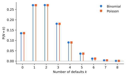
Example 9 A bank holds n = 500 independent loans, each with a default probability of p = 0.004 over the next year. The expected number of defaults is \lambda = n p = 2. The exact probability of no defaults is \operatorname{P}(N = 0) = (1 - 0.004)^{500} = 0.1348, while the Poisson approximation gives e^{-2} = 0.1353. Similarly, the probability of exactly three defaults is 0.1808 under the binomial distribution and 0.1804 under the Poisson approximation. Figure 1 shows that the two distributions are nearly indistinguishable.
The Poisson limit is the first of two limits of sums of Bernoulli random variables that we will study. Here the number of trials grows while each success becomes rare, and the limit is a count. In the notes on Brownian motion, the number of coin flips also grows but each flip is scaled down in size, and the limit is a normal random variable. The first limit leads to the Poisson process and the second to Brownian motion.
Moment Generating Functions
Definition
The PGF only makes sense for random variables that take values in \mathbb{N}. To handle random variables with negative or continuous values, such as stock returns, we substitute z = e^{\theta} in the definition of the PGF. The moment generating function of a random variable X is M_{X}(\theta) = \operatorname{E}(e^{\theta X}), defined for all real \theta such that the expectation is finite. If X takes values in \mathbb{N}, then M_{X}(\theta) = G_{X}(e^{\theta}). If X has a probability density function f, the expectation is an integral, M_{X}(\theta) = \int_{-\infty}^{\infty} e^{\theta x} f(x) \, dx. We always have M_{X}(0) = 1.
We have in fact already computed an MGF. In the notes on continuous distributions we showed that if X \sim \mathcal{N}(\mu, \sigma^{2}), then \operatorname{E}(e^{\alpha X}) = e^{\alpha \mu + \frac{1}{2} \alpha^{2} \sigma^{2}} for any real \alpha, and used this expression to find the moments of a lognormal random variable. That calculation was the MGF of the normal distribution evaluated at \theta = \alpha. Below we see that it is one instance of a general method.
The name comes from the power series of the exponential function. Since e^{\theta X} = 1 + \theta X + \frac{\theta^{2}}{2!} X^{2} + \frac{\theta^{3}}{3!} X^{3} + \cdots, taking expectations term by term gives M_{X}(\theta) = 1 + \theta \operatorname{E}(X) + \frac{\theta^{2}}{2!} \operatorname{E}(X^{2}) + \frac{\theta^{3}}{3!} \operatorname{E}(X^{3}) + \cdots, so the moments of X are the coefficients of the series.
The second property follows from e^{\theta (a + b X)} = e^{a \theta} e^{(b \theta) X}, and the third from the same argument we used for the PGF. The first and fourth require more work, and we take them as given.
The Exponential and Gamma Distributions
Recall from the notes on continuous distributions that T \sim \text{Exp}(\lambda) has density \lambda e^{-\lambda t} for t \geq 0, and that X \sim \text{Gamma}(\alpha, \lambda) has density \lambda^{\alpha} x^{\alpha - 1} e^{-\lambda x} / \Gamma(\alpha) for x > 0, with \text{Gamma}(1, \lambda) = \text{Exp}(\lambda).
Example 10 For \theta < \lambda, the MGF of T \sim \text{Exp}(\lambda) is M_{T}(\theta) = \int_{0}^{\infty} e^{\theta t} \lambda e^{-\lambda t} \, dt = \lambda \int_{0}^{\infty} e^{-(\lambda - \theta) t} \, dt = \frac{\lambda}{\lambda - \theta}. For \theta \geq \lambda the integral diverges, so the MGF is only finite on the interval (-\infty, \lambda). Differentiating, M_{T}'(\theta) = \frac{\lambda}{(\lambda - \theta)^{2}}, \qquad M_{T}''(\theta) = \frac{2 \lambda}{(\lambda - \theta)^{3}}, so that \operatorname{E}(T) = 1 / \lambda, \operatorname{E}(T^{2}) = 2 / \lambda^{2}, and \operatorname{V}(T) = 1 / \lambda^{2}, without computing any integral by parts.
Example 11 For X \sim \text{Gamma}(\alpha, \lambda) and \theta < \lambda, the integrand of the MGF is proportional to a gamma density with rate \lambda - \theta, so that M_{X}(\theta) = \frac{\lambda^{\alpha}}{\Gamma(\alpha)} \int_{0}^{\infty} x^{\alpha - 1} e^{-(\lambda - \theta) x} \, dx = \frac{\lambda^{\alpha}}{\Gamma(\alpha)} \frac{\Gamma(\alpha)}{(\lambda - \theta)^{\alpha}} = \left(\frac{\lambda}{\lambda - \theta}\right)^{\alpha}.
The MGF of the gamma distribution is the MGF of the exponential distribution raised to the power \alpha. Together with the product rule for sums, this gives three useful results.
First, let T_{1}, T_{2}, \ldots, T_{n} be independent \text{Exp}(\lambda) random variables and let W_{n} = T_{1} + \cdots + T_{n}. Then M_{W_{n}}(\theta) = \left(\frac{\lambda}{\lambda - \theta}\right)^{n}, \qquad \theta < \lambda, which is the MGF of a \text{Gamma}(n, \lambda) random variable. By uniqueness, the sum of n independent exponential waiting times has a gamma distribution with shape n. In a Poisson process, W_{n} is the time at which the n-th event occurs.
Second, the same argument shows that if X_{1} \sim \text{Gamma}(\alpha_{1}, \lambda) and X_{2} \sim \text{Gamma}(\alpha_{2}, \lambda) are independent with the same rate, then X_{1} + X_{2} \sim \text{Gamma}(\alpha_{1} + \alpha_{2}, \lambda).
Third, the notes on continuous distributions show that the square of a standard normal random variable has a \text{Gamma}(1/2, 1/2) distribution. If Z_{1}, \ldots, Z_{k} are independent standard normal random variables, the second result implies that Z_{1}^{2} + \cdots + Z_{k}^{2} \sim \text{Gamma}(k / 2, 1 / 2), which is the chi-squared distribution with k degrees of freedom. Its MGF is (1 - 2 \theta)^{-k/2} for \theta < 1/2, and its mean and variance are k and 2 k.
The Normal Distribution
Recall from the notes on continuous distributions that X \sim \mathcal{N}(\mu, \sigma^{2}) can be written as X = \mu + \sigma Z, where Z has the standard normal density f(z) = e^{-\frac{1}{2} z^{2}} / \sqrt{2 \pi}. We now state the MGF of the normal distribution in the language of this chapter. Working with Z first and then using the properties of the MGF shortens the calculation, and the same pattern will give us the characteristic function below.
Proof
We first compute the MGF of Z \sim \mathcal{N}(0, 1). Completing the square in the exponent, \theta z - \frac{1}{2} z^{2} = -\frac{1}{2} (z - \theta)^{2} + \frac{1}{2} \theta^{2}, so that M_{Z}(\theta) = \int_{-\infty}^{\infty} \frac{1}{\sqrt{2 \pi}} e^{\theta z - \frac{1}{2} z^{2}} \, dz = e^{\frac{1}{2} \theta^{2}} \underbrace{\int_{-\infty}^{\infty} \frac{1}{\sqrt{2 \pi}} e^{-\frac{1}{2} (z - \theta)^{2}} \, dz}_{= 1} = e^{\frac{1}{2} \theta^{2}}. The integral equals one because the integrand is the density of a normal random variable with mean \theta and variance one. Since X = \mu + \sigma Z, the second property of the MGF gives M_{X}(\theta) = e^{\mu \theta} M_{Z}(\sigma \theta) = e^{\mu \theta + \frac{1}{2} \sigma^{2} \theta^{2}}.Equation (2) has two immediate consequences. First, if X_{1} \sim \mathcal{N}(\mu_{1}, \sigma_{1}^{2}) and X_{2} \sim \mathcal{N}(\mu_{2}, \sigma_{2}^{2}) are independent, then M_{X_{1} + X_{2}}(\theta) = e^{(\mu_{1} + \mu_{2}) \theta + \frac{1}{2} (\sigma_{1}^{2} + \sigma_{2}^{2}) \theta^{2}}, so by uniqueness X_{1} + X_{2} \sim \mathcal{N}(\mu_{1} + \mu_{2}, \sigma_{1}^{2} + \sigma_{2}^{2}). Sums of independent normal random variables are normal. This is why, in a model where daily log returns are independent and normal, annual log returns are also normal.
Second, we recover the lognormal moments from the notes on continuous distributions. If Y = e^{X}, every moment of Y is a value of the MGF of X, \operatorname{E}(Y^{\alpha}) = \operatorname{E}(e^{\alpha X}) = M_{X}(\alpha) = e^{\alpha \mu + \frac{1}{2} \alpha^{2} \sigma^{2}}, so \operatorname{E}(Y) = M_{X}(1) and \operatorname{E}(Y^{2}) = M_{X}(2). There we found \operatorname{E}(Y) by completing the square inside an integral. Here every moment follows by evaluating one function at different points.
Example 12 Suppose the log return of a stock over the next year is X \sim \mathcal{N}(\mu, \sigma^{2}) with \mu = 0.08 and \sigma = 0.20, so that the stock price in one year is S_{1} = S_{0} e^{X}. The expected gross return is \operatorname{E}\left(\frac{S_{1}}{S_{0}}\right) = M_{X}(1) = e^{0.08 + \frac{1}{2} (0.20)^{2}} = e^{0.10} = 1.1052. The expected simple return of 10.52% exceeds e^{0.08} - 1 = 8.33\%, the simple return at the mean log return. The difference comes from the term \frac{1}{2} \sigma^{2}, the same correction that will appear in Itô’s lemma.
Cumulant Generating Functions
It is often convenient to work with the logarithm of the MGF, K_{X}(\theta) = \ln M_{X}(\theta), called the cumulant generating function. Since the MGF of a sum of independent random variables is a product, the cumulant generating function of the sum is a sum, K_{X + Y}(\theta) = K_{X}(\theta) + K_{Y}(\theta). Its first two derivatives at zero are the mean and the variance: K_{X}'(0) = \frac{M_{X}'(0)}{M_{X}(0)} = \operatorname{E}(X), \qquad K_{X}''(0) = \frac{M_{X}''(0) M_{X}(0) - M_{X}'(0)^{2}}{M_{X}(0)^{2}} = \operatorname{E}(X^{2}) - \operatorname{E}(X)^{2} = \operatorname{V}(X).
For the two distributions that drive this course, the cumulant generating functions are particularly simple: X \sim \mathcal{N}(\mu, \sigma^{2}) : \quad K_{X}(\theta) = \mu \theta + \tfrac{1}{2} \sigma^{2} \theta^{2}, \qquad N \sim \text{Poisson}(\lambda) : \quad K_{N}(\theta) = \lambda (e^{\theta} - 1). The derivatives K_{X}^{(k)}(0) are called the cumulants of X. The normal cumulant generating function is a quadratic, so all cumulants beyond the variance are zero. The Poisson one is linear in \lambda, which reflects the fact that Poisson counts over disjoint periods add up.
The cumulant generating function also produces martingales. If X_{1}, X_{2}, \ldots are iid with cumulant generating function K and S_{n} = X_{1} + \cdots + X_{n}, then each factor e^{\theta X_{i} - K(\theta)} is positive with expectation one, so their product M_{n} = e^{\theta S_{n} - n K(\theta)} is a martingale of the type studied in the notes on discrete-time martingales. These exponential martingales will allow us to compute the distribution of stopping times and to change probability measures.
When the MGF Does Not Exist
The MGF requires \operatorname{E}(e^{\theta X}) to be finite, and for some random variables this fails for every \theta > 0. The lognormal distribution is the most important example in finance. If Y = e^{X} with X normal, all moments \operatorname{E}(Y^{k}) = e^{k \mu + \frac{1}{2} k^{2} \sigma^{2}} are finite, but they grow so fast that the series \sum_{k} \theta^{k} \operatorname{E}(Y^{k}) / k! diverges for any \theta > 0. Equivalently, e^{\theta e^{x}} grows faster than the normal density decays, so \operatorname{E}(e^{\theta Y}) = \infty. The MGF of a stock price in the Black-Scholes model does not exist, even though the MGF of its logarithm does.
The same problem arises with heavy-tailed distributions, such as the Student t distribution, whose moments are infinite beyond some order. To handle all random variables with a single tool we need a transform that is always finite.
Characteristic Functions
Definition
The characteristic function of a random variable X is \phi_{X}(u) = \operatorname{E}(e^{i u X}), \qquad u \in \mathbb{R}, where i is the imaginary unit, i^{2} = -1. By Euler’s formula, e^{i u x} = \cos(u x) + i \sin(u x), so the characteristic function is \phi_{X}(u) = \operatorname{E}(\cos(u X)) + i \, \operatorname{E}(\sin(u X)). Both expectations are finite because the sine and cosine are bounded by one. Therefore, unlike the MGF, the characteristic function exists for every random variable and every real u.
The characteristic function is the MGF evaluated at an imaginary argument. When the MGF is finite around zero, replacing \theta by i u in its formula gives \phi_{X}(u), although justifying this step requires complex analysis. For random variables in \mathbb{N} the relation is direct, \phi_{X}(u) = G_{X}(e^{i u}). The three transforms are therefore the same object seen from different angles: \phi_{X}(u) = \operatorname{E}(e^{i u X}), \qquad M_{X}(\theta) = \operatorname{E}(e^{\theta X}), \qquad G_{X}(z) = \operatorname{E}(z^{X}).
The bound |\phi_{X}(u)| \leq \operatorname{E}(|e^{i u X}|) = 1 holds because |e^{i u x}| = \sqrt{\cos^{2}(u x) + \sin^{2}(u x)} = 1. The second and third properties follow exactly as for the MGF. In particular, \operatorname{E}(X) = -i \phi_{X}'(0) and \operatorname{E}(X^{2}) = -\phi_{X}''(0).
Example 13 If N \sim \text{Poisson}(\lambda), then \phi_{N}(u) = G_{N}(e^{i u}) = e^{\lambda (e^{i u} - 1)}.
Example 14 If X takes the values 1 and -1 with probability 1/2 each, then \phi_{X}(u) = \frac{1}{2} e^{i u} + \frac{1}{2} e^{-i u} = \cos(u). The characteristic function is real because the distribution of X is symmetric around zero, so the sine terms cancel.
The Normal Characteristic Function
Replacing \theta by i u in (2) suggests that the characteristic function of X \sim \mathcal{N}(\mu, \sigma^{2}) is e^{i \mu u - \frac{1}{2} \sigma^{2} u^{2}}. The following argument confirms it without complex analysis.
Proof
Let Z \sim \mathcal{N}(0, 1) with density f(z) = e^{-\frac{1}{2} z^{2}} / \sqrt{2 \pi}, and note that f'(z) = -z f(z). Differentiating \phi_{Z}(u) = \int e^{i u z} f(z) \, dz under the integral sign, \phi_{Z}'(u) = \int_{-\infty}^{\infty} i z e^{i u z} f(z) \, dz = -i \int_{-\infty}^{\infty} e^{i u z} f'(z) \, dz. Integrating by parts, and using that f(z) \to 0 as |z| \to \infty, \phi_{Z}'(u) = -i \left( \left. e^{i u z} f(z) \right|_{-\infty}^{\infty} - \int_{-\infty}^{\infty} i u \, e^{i u z} f(z) \, dz \right) = i^{2} u \, \phi_{Z}(u) = -u \, \phi_{Z}(u). The solution of this differential equation with \phi_{Z}(0) = 1 is \phi_{Z}(u) = e^{-\frac{1}{2} u^{2}}. Since X = \mu + \sigma Z, the second property of the characteristic function gives \phi_{X}(u) = e^{i \mu u} \phi_{Z}(\sigma u) = e^{i \mu u - \frac{1}{2} \sigma^{2} u^{2}}.Recovering Probabilities
Uniqueness says that the characteristic function determines the distribution, but it is also possible to recover probabilities from it explicitly. For random variables taking integer values the formula is simple.
Proof
Writing \phi_{X}(u) = \sum_{j} p_{X}(j) e^{i u j} and integrating term by term, \frac{1}{2 \pi} \int_{-\pi}^{\pi} e^{-i u k} \phi_{X}(u) \, du = \sum_{j} p_{X}(j) \frac{1}{2 \pi} \int_{-\pi}^{\pi} e^{i u (j - k)} \, du. If j = k the integrand is one and the integral equals 2 \pi. If j \neq k, the integral of \cos(u (j - k)) and \sin(u (j - k)) over a full period is zero. Therefore only the term j = k survives, and it equals p_{X}(k).A similar formula holds for continuous random variables, where the density is recovered as f(x) = \frac{1}{2 \pi} \int_{-\infty}^{\infty} e^{-i u x} \phi_{X}(u) \, du whenever the integral converges. This is the Fourier inversion formula. It is the basis of the option pricing methods used in practice for models where the density of the stock price is unknown but its characteristic function has a closed form.
Convergence in Distribution
The main use of characteristic functions is to prove limit theorems. We say that a sequence of random variables X_{n} converges in distribution to X if \operatorname{P}(X_{n} \leq x) \to \operatorname{P}(X \leq x) at every point x where the cumulative distribution function of X is continuous. The following theorem, which we state without proof, reduces convergence in distribution to the convergence of a sequence of functions.
This theorem plays the same role for general random variables that the continuity theorem for PGFs played for counts. Its most important application is the central limit theorem.
Proof
Since \operatorname{E}(X_{1}) = 0 and \operatorname{E}(X_{1}^{2}) = \sigma^{2}, the fourth property of the characteristic function gives \phi_{X_{1}}'(0) = 0 and \phi_{X_{1}}''(0) = -\sigma^{2}. A second-order Taylor expansion around zero then yields \phi_{X_{1}}(u) = 1 - \frac{1}{2} \sigma^{2} u^{2} + o(u^{2}), where o(u^{2}) denotes terms that vanish faster than u^{2} as u \to 0. Using the second and third properties, \phi_{S_{n} / \sqrt{n}}(u) = \phi_{X_{1}}\left(\frac{u}{\sqrt{n}}\right)^{n} = \left(1 - \frac{\sigma^{2} u^{2}}{2 n} + o\left(\frac{1}{n}\right)\right)^{n} \xrightarrow[n \to \infty]{} e^{-\frac{1}{2} \sigma^{2} u^{2}}. The limit is the characteristic function of \mathcal{N}(0, \sigma^{2}), and Lévy’s continuity theorem completes the proof.The structure of the proof mirrors the Poisson limit. In both cases we raise the transform of a single term to the n-th power and use (1 + x / n)^{n} \to e^{x}. In the Poisson limit each term is a rare event with probability \lambda / n. In the central limit theorem each term is a small shock of size 1 / \sqrt{n}. The notes on Brownian motion apply this argument to a random walk with steps \pm \sqrt{\Delta t}, using the characteristic function \cos(u \sqrt{\Delta t}) from Example 14.
Summary
The table below collects the transforms of the distributions used in these notes. The MGFs of the geometric distribution and of the exponential and gamma distributions are finite only for \theta < -\ln(1 - p) and \theta < \lambda, respectively. The characteristic function of each can be obtained from its MGF by setting \theta = i u.
| Distribution | Support | PGF G(z) | MGF M(\theta) | Mean | Variance |
|---|---|---|---|---|---|
| Bernoulli(p) | \{0, 1\} | 1 - p + p z | 1 - p + p e^{\theta} | p | p (1 - p) |
| Binomial(n, p) | \{0, \ldots, n\} | (1 - p + p z)^{n} | (1 - p + p e^{\theta})^{n} | n p | n p (1 - p) |
| Geometric(p) | \{1, 2, \ldots\} | \frac{p z}{1 - (1 - p) z} | \frac{p e^{\theta}}{1 - (1 - p) e^{\theta}} | \frac{1}{p} | \frac{1 - p}{p^{2}} |
| Poisson(\lambda) | \{0, 1, \ldots\} | e^{\lambda (z - 1)} | e^{\lambda (e^{\theta} - 1)} | \lambda | \lambda |
| Exp(\lambda) | [0, \infty) | \frac{\lambda}{\lambda - \theta} | \frac{1}{\lambda} | \frac{1}{\lambda^{2}} | |
| Gamma(\alpha, \lambda) | (0, \infty) | \left(\frac{\lambda}{\lambda - \theta}\right)^{\alpha} | \frac{\alpha}{\lambda} | \frac{\alpha}{\lambda^{2}} | |
| \mathcal{N}(\mu, \sigma^{2}) | \mathbb{R} | e^{\mu \theta + \frac{1}{2} \sigma^{2} \theta^{2}} | \mu | \sigma^{2} |
Looking Ahead: The Ruin Problem
Consider a random walk whose steps X_{i} take the value +1 with probability p and -1 with probability q = 1 - p. The steps take negative values, so they have no PGF in the strict sense, but \operatorname{E}(z^{X}) = p z + q / z is still well defined for z > 0. Setting this expression equal to one, p z + \frac{q}{z} = 1 \quad \Longleftrightarrow \quad p z^{2} - z + q = 0, gives the roots z = 1 and z = q / p. Whenever \operatorname{E}(z^{X}) = 1, the process z^{S_{n}} is a martingale, which is why the notes on ruin probabilities try solutions of the form f(K) = z^{K}. When p \neq q the second root q / p gives the ruin probabilities for a biased coin. When p = q = 1/2 the equation becomes (z - 1)^{2} = 0 and both roots equal one, so z^{K} only produces the constant solution. The second solution is f(K) = K, which comes from the fact that the position S_{n} of a symmetric walk is itself a martingale. We will develop this connection in the notes on ruin probabilities and on martingales.