Continuous Distributions

The notes on probability basics worked with random variables that take a countable number of values, described by a probability mass function. Many quantities in finance, such as returns, prices, and waiting times, are better modeled as taking any value in an interval. These notes introduce continuous random variables and the distributions used most often in the rest of the course.

We start with the uniform distribution, which is the basis of simulation, and the exponential and gamma distributions, which describe waiting times and reappear in the Poisson process. We then study the normal distribution in detail, together with the chi-squared distribution of its square, and the lognormal distribution used to model stock prices. We close with the bivariate normal distribution, which describes correlated returns, and with the Student t distribution, the simplest model of the heavy tails observed in financial data.

Continuous Random Variables

A continuous random variable X is described by a probability density function (PDF) f(x) \geq 0 with \int_{-\infty}^{\infty} f(x) \, dx = 1, so that probabilities are areas under the density, \operatorname{P}(a < X \leq b) = \int_{a}^{b} f(x) \, dx. The density is not a probability. It can exceed one, and f(x) \, dx is approximately the probability that X falls in a short interval of length dx around x. In particular, the probability that X takes any single value is zero, so it does not matter whether we include the endpoints of an interval.

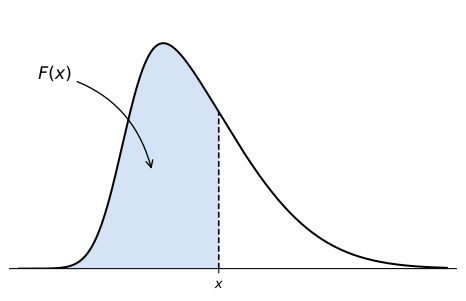
The cumulative distribution function (CDF) of X is F(x) = \operatorname{P}(X \leq x) = \int_{-\infty}^{x} f(u) \, du. It increases from 0 to 1, and by the fundamental theorem of calculus F'(x) = f(x) wherever f is continuous. Geometrically, F(x) is the area under the density to the left of x, as Figure 1 shows.

Figure 1: The shaded area under the density f to the left of x is the cumulative probability F(x) = \operatorname{P}(X \leq x).

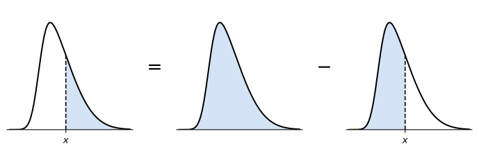
The CDF is all we need to compute the probability of any interval. Since \operatorname{P}(X \leq x) + \operatorname{P}(X > x) = 1, the probability of the right tail, also called the survival function, is \operatorname{P}(X > x) = 1 - F(x). In words, the area to the right of x is the total area, which is one, minus the area to the left of x, as Figure 2 shows.

Figure 2: The right-tail probability is the probability of the whole distribution, which is one, minus the left-tail probability.

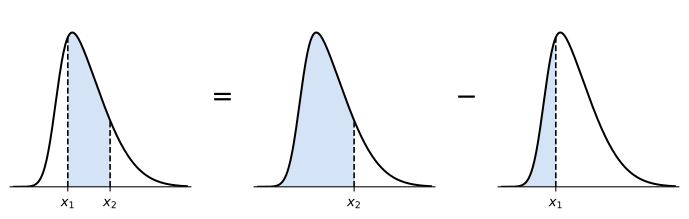
Similarly, the probability that X falls within an interval (x_{1}, x_{2}] is the area to the left of x_{2} minus the area to the left of x_{1}, \operatorname{P}(x_{1} < X \leq x_{2}) = F(x_{2}) - F(x_{1}), as Figure 3 shows.

Figure 3: If you subtract the area to the left of x_{1} from the area to the left of x_{2} you obtain the probability of x_{1} < X \leq x_{2}.

Both identities hold for every continuous distribution, symmetric or not.

Sums over the support become integrals, and the expectation of a function of X is \operatorname{E}(g(X)) = \int_{-\infty}^{\infty} g(x) f(x) \, dx, provided the integral converges absolutely. In particular, \operatorname{E}(X) = \int x f(x) \, dx and \operatorname{V}(X) = \operatorname{E}(X^{2}) - \operatorname{E}(X)^{2}. All the results in the notes on probability basics and on conditioning and independence carry over with this replacement. For example, two continuous random variables with joint density f(x, y) are independent if f(x, y) = f_{X}(x) f_{Y}(y), and the expectation of a product of independent random variables is the product of their expectations.

Many distributions in these notes are obtained by transforming a simpler random variable. If Y = g(X) where g is strictly increasing, then \operatorname{P}(Y \leq y) = \operatorname{P}(X \leq g^{-1}(y)), and differentiating gives the density of Y, f_{Y}(y) = f_{X}(g^{-1}(y)) \, \frac{d g^{-1}(y)}{d y}. \tag{1} The derivative accounts for the stretching or compression of intervals under the transformation.

The Uniform Distribution

A random variable U is uniformly distributed on the interval [a, b] if its density is constant on the interval, f(u) = \frac{1}{b - a}, \qquad a \leq u \leq b, and zero elsewhere. We write U \sim \text{Uniform}(a, b). Every subinterval of the same length has the same probability, and \operatorname{P}(U \leq u) = (u - a) / (b - a) for a \leq u \leq b.

WarningMoments of the Uniform Distribution

If U \sim \text{Uniform}(a, b), then \operatorname{E}(U) = \frac{a + b}{2}, \qquad \operatorname{V}(U) = \frac{(b - a)^{2}}{12}.

Proof

We have \begin{aligned} \operatorname{E}(U) & = \int_{a}^{b} \frac{u}{b - a} \, du = \frac{b^{2} - a^{2}}{2 (b - a)} = \frac{a + b}{2}, \\ \operatorname{E}(U^{2}) & = \int_{a}^{b} \frac{u^{2}}{b - a} \, du = \frac{b^{3} - a^{3}}{3 (b - a)} = \frac{a^{2} + a b + b^{2}}{3}. \end{aligned} Therefore, \operatorname{V}(U) = \frac{a^{2} + a b + b^{2}}{3} - \frac{(a + b)^{2}}{4} = \frac{a^{2} - 2 a b + b^{2}}{12} = \frac{(b - a)^{2}}{12}.

The uniform distribution on [0, 1] is the starting point of every simulation. Computers generate numbers that behave like independent draws from \text{Uniform}(0, 1), and the following result turns them into draws from any other distribution.

WarningInverse Transform Method

Let F be a continuous and strictly increasing CDF, and let U \sim \text{Uniform}(0, 1). Then the random variable X = F^{-1}(U) has CDF F.

Proof

Since F is strictly increasing, F^{-1}(U) \leq x if and only if U \leq F(x). Therefore, \operatorname{P}(X \leq x) = \operatorname{P}(U \leq F(x)) = F(x), where the last step uses \operatorname{P}(U \leq u) = u for 0 \leq u \leq 1.

We apply this method to the exponential distribution in the next section.

The Exponential Distribution

A random variable T has an exponential distribution with rate \lambda > 0 if its density is f(t) = \lambda e^{-\lambda t}, \qquad t \geq 0, and we write T \sim \text{Exp}(\lambda). The exponential distribution describes the waiting time until an event that occurs at a constant rate \lambda per unit of time, such as the time until a firm defaults when its default intensity is constant, or the time until the next trade in a stock. Integrating the density, the CDF and the survival function are F(t) = 1 - e^{-\lambda t}, \qquad \operatorname{P}(T > t) = e^{-\lambda t}.

WarningMoments of the Exponential Distribution

If T \sim \text{Exp}(\lambda), then \operatorname{E}(T) = \frac{1}{\lambda}, \qquad \operatorname{V}(T) = \frac{1}{\lambda^{2}}.

Proof

Integrating by parts with u = t and dv = \lambda e^{-\lambda t} dt, \operatorname{E}(T) = \int_{0}^{\infty} t \lambda e^{-\lambda t} \, dt = \left. -t e^{-\lambda t} \right|_{0}^{\infty} + \int_{0}^{\infty} e^{-\lambda t} \, dt = \frac{1}{\lambda}. Similarly, \operatorname{E}(T^{2}) = \int_{0}^{\infty} t^{2} \lambda e^{-\lambda t} \, dt = \left. -t^{2} e^{-\lambda t} \right|_{0}^{\infty} + 2 \int_{0}^{\infty} t e^{-\lambda t} \, dt = \frac{2}{\lambda} \operatorname{E}(T) = \frac{2}{\lambda^{2}}, so that \operatorname{V}(T) = 2 / \lambda^{2} - 1 / \lambda^{2} = 1 / \lambda^{2}.

Example 1 Suppose a firm defaults at an exponentially distributed time with intensity \lambda = 0.02 per year. The probability that it defaults within ten years is \operatorname{P}(T \leq 10) = 1 - e^{-0.02 \times 10} = 0.1813. The expected time to default is 1 / \lambda = 50 years, but the median time to default, which solves 1 - e^{-\lambda t} = 1/2, is \ln(2) / \lambda = 34.66 years. The mean exceeds the median because the long right tail of the distribution pulls the mean up.

The exponential distribution has a special property: having waited s units of time without an event does not change the distribution of the remaining waiting time. This memoryless property is what makes it the natural model for waiting times in the Poisson process, and we study it in the notes on Poisson processes.

To simulate an exponential random variable with the inverse transform method, we solve u = 1 - e^{-\lambda t} for t to find F^{-1}(u) = -\ln(1 - u) / \lambda. Since 1 - U is also uniform on [0, 1], we can equally use T = -\ln(U) / \lambda. The following code simulates 100,000 exponential waiting times with \lambda = 2 and compares their sample mean and variance with the theoretical values 1 / \lambda = 0.5 and 1 / \lambda^{2} = 0.25.

import numpy as np

rng = np.random.default_rng(42)
lam = 2.0
u = rng.uniform(size=100_000)
t = -np.log(u) / lam
print(t.mean(), t.var())

0.4996447052680305 0.2519802306340005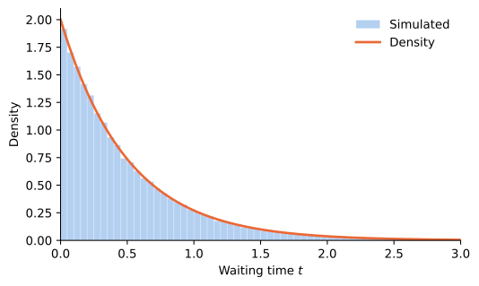

Figure 4: The figure compares a histogram of 100,000 simulated waiting times T = -\ln(U) / \lambda with the exponential density \lambda e^{-\lambda t} for \lambda = 2.

The Gamma Distribution

The exponential distribution describes the waiting time for one event. The gamma distribution generalizes it, and it describes, among other things, the waiting time for several events. Its density involves the gamma function \Gamma(\alpha) = \int_{0}^{\infty} x^{\alpha - 1} e^{-x} \, dx, \qquad \alpha > 0. Integrating by parts shows that \Gamma(\alpha + 1) = \alpha \Gamma(\alpha), and since \Gamma(1) = 1, we have \Gamma(n) = (n - 1)! for every positive integer n. The gamma function therefore extends the factorial to non-integer arguments. We will also need the value \Gamma(1/2) = \sqrt{\pi}.

A random variable X has a gamma distribution with shape \alpha > 0 and rate \lambda > 0 if its density is f(x) = \frac{\lambda^{\alpha}}{\Gamma(\alpha)} x^{\alpha - 1} e^{-\lambda x}, \qquad x > 0, and we write X \sim \text{Gamma}(\alpha, \lambda). The substitution u = \lambda x and the definition of \Gamma(\alpha) show that the density integrates to one. With \alpha = 1 we recover the exponential distribution, \text{Gamma}(1, \lambda) = \text{Exp}(\lambda).

WarningMoments of the Gamma Distribution

If X \sim \text{Gamma}(\alpha, \lambda), then \operatorname{E}(X) = \frac{\alpha}{\lambda}, \qquad \operatorname{V}(X) = \frac{\alpha}{\lambda^{2}}.

Proof

For any k \geq 1, the integrand of \operatorname{E}(X^{k}) is proportional to a gamma density with shape \alpha + k, so that \operatorname{E}(X^{k}) = \frac{\lambda^{\alpha}}{\Gamma(\alpha)} \int_{0}^{\infty} x^{\alpha + k - 1} e^{-\lambda x} \, dx = \frac{\lambda^{\alpha}}{\Gamma(\alpha)} \frac{\Gamma(\alpha + k)}{\lambda^{\alpha + k}} = \frac{\Gamma(\alpha + k)}{\Gamma(\alpha) \lambda^{k}}. Using \Gamma(\alpha + 1) = \alpha \Gamma(\alpha) and \Gamma(\alpha + 2) = (\alpha + 1) \alpha \Gamma(\alpha), we find \operatorname{E}(X) = \alpha / \lambda and \operatorname{E}(X^{2}) = \alpha (\alpha + 1) / \lambda^{2}, so that \operatorname{V}(X) = \alpha / \lambda^{2}.

The shape parameter controls the form of the density, as Figure 5 shows. For \alpha \leq 1 the density decreases from its value at zero, which is infinite when \alpha < 1, while for \alpha > 1 it rises from zero to a peak at (\alpha - 1) / \lambda and then decays. The rate parameter only rescales the horizontal axis.

Figure 5: The figure plots gamma densities with rate \lambda = 1 and shapes \alpha = 1, 2, and 4. The case \alpha = 1 is the exponential distribution.

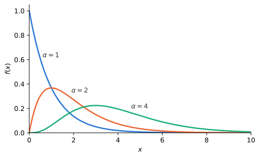
The notes on generating functions show that the sum of n independent \text{Exp}(\lambda) random variables has a \text{Gamma}(n, \lambda) distribution. In a Poisson process with rate \lambda, the waiting times between events are exponential, so the time of the n-th event is gamma distributed with shape n. The gamma distribution also appears as the long-run distribution of the short rate in the Cox-Ingersoll-Ross model of interest rates.

The Normal Distribution

We say that a real-valued random variable X is normally distributed with mean \mu and standard deviation \sigma if its density is f(x) = \frac{1}{\sqrt{2 \pi \sigma^{2}}} e^{-\frac{(x - \mu)^{2}}{2 \sigma^{2}}}, and we write X \sim \mathcal{N}(\mu, \sigma^{2}). The parameters \mu and \sigma are related to the first and second moments of X.

Figure 6: The figure shows the density function of a normally distributed random variable with mean \mu and standard deviation \sigma.

WarningMoments of the Normal Distribution

The parameter \mu is the mean or expectation of X while \sigma denotes its standard deviation. The variance of X is given by \sigma^{2}.

Proof

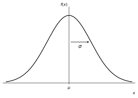
Let X = \mu + \sigma Z where Z \sim \mathcal{N}(0, 1), and let f(z) = e^{-\frac{1}{2} z^{2}} / \sqrt{2 \pi} be the density of Z, which satisfies f'(z) = -z f(z). Since f(z) \to 0 and z f(z) \to 0 as |z| \to \infty, \begin{aligned} \operatorname{E}(Z) & = \int_{-\infty}^{\infty} z f(z) \, dz = -\int_{-\infty}^{\infty} f'(z) \, dz = \left. -f(z) \right|_{-\infty}^{\infty} = 0, \\ \operatorname{E}(Z^{2}) & = \int_{-\infty}^{\infty} z \cdot z f(z) \, dz = -\int_{-\infty}^{\infty} z f'(z) \, dz \\ & = \left. -z f(z) \right|_{-\infty}^{\infty} + \int_{-\infty}^{\infty} f(z) \, dz = 0 + 1 = 1, \end{aligned} where the second line integrates by parts and uses that a density integrates to one. Therefore, \operatorname{V}(Z) = \operatorname{E}(Z^{2}) - \operatorname{E}(Z)^{2} = 1.

We can now compute \operatorname{E}(X) = \mu + \sigma \operatorname{E}(Z) = \mu and \operatorname{V}(X) = \sigma^{2} \operatorname{V}(Z) = \sigma^{2}.

The Standard Normal Distribution

An important case of normally distributed random variables is when \mu = 0 and \sigma = 1. In this case we say that Z \sim \mathcal{N}(0, 1) has the standard normal distribution and its cumulative distribution function is usually denoted by the capital Greek letter \Phi (phi), and is defined by the integral: \mathop{\Phi}(z) = \operatorname{P}(Z \leq z) = \int_{-\infty}^{z} \frac{1}{\sqrt{2 \pi}} e^{-\frac{x^{2}}{2}} \, dx.

The normal density is symmetric around zero, so the area to the left of -z equals the area to the right of z, as Figure 7 shows. Combined with the right-tail identity, this gives \mathop{\Phi}(-z) = \operatorname{P}(Z \leq -z) = \operatorname{P}(Z > z) = 1 - \mathop{\Phi}(z). \tag{2} Therefore we only need the values of \mathop{\Phi}(z) for z \geq 0, which is why printed normal tables list only positive values, and every left-tail probability of a standard normal random variable can be turned into a right-tail probability and vice versa.

Figure 7: By the symmetry of the standard normal density, the area to the left of -z, which is \mathop{\Phi}(-z), equals the area to the right of z, which is 1 - \mathop{\Phi}(z).

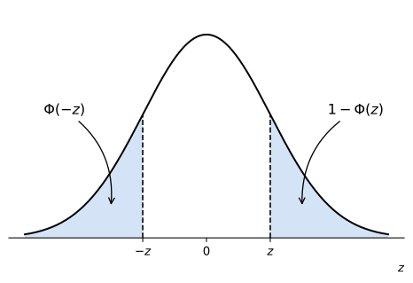
Since the integral that defines \mathop{\Phi}(z) cannot be solved in closed form, its values must be obtained from a table or using a computer. For example, in Python we can compute \mathop{\Phi}(-0.4) with the norm object from the scipy.stats library:

from scipy.stats import norm

print(norm.cdf(-0.4))

0.3445782583896758

If you prefer to use Excel, you need to type in a cell =norm.s.dist(-0.4,TRUE), which yields the same answer. By (2), 1 - \mathop{\Phi}(0.4) gives the same value.

Computing Normal Probabilities

Knowing how to compute \mathop{\Phi}(z) allows us to compute probabilities for any normal random variable. If X \sim \mathcal{N}(\mu, \sigma^{2}), then Z = \frac{X - \mu}{\sigma} \sim \mathcal{N}(0, 1), so that \operatorname{P}(X \leq x) = \operatorname{P}\left( \frac{X - \mu}{\sigma} \leq \frac{x - \mu}{\sigma} \right) = \mathop{\Phi}\left(\frac{x - \mu}{\sigma}\right). The standardized value Z = \dfrac{X - \mu}{\sigma} is called a Z-score. Right-tail and interval probabilities then follow from the general identities \operatorname{P}(X > x) = 1 - F(x) and \operatorname{P}(x_{1} < X \leq x_{2}) = F(x_{2}) - F(x_{1}) with F(x) = \mathop{\Phi}((x - \mu) / \sigma).

Example 2 Suppose that X \sim \mathcal{N}(\mu, \sigma^{2}) with \mu = 10 and \sigma = 25. What is the probability that X \leq 0? \operatorname{P}(X \leq 0) = \operatorname{P}\left( Z \leq \tfrac{0 - 10}{25} \right) = \mathop{\Phi}(-0.40) = 0.3446.

Example 3 Suppose that X \sim \mathcal{N}(\mu, \sigma^{2}) with \mu = 10 and \sigma = 25. What is the probability that X > 12? We first compute the left-tail probability, \operatorname{P}(X \leq 12) = \operatorname{P}\left( Z \leq \tfrac{12 - 10}{25} \right) = \mathop{\Phi}(0.08) = 0.5319. Therefore, \operatorname{P}(X > 12) = 1 - 0.5319 = 0.4681.

Example 4 Suppose that X \sim \mathcal{N}(\mu, \sigma^{2}) with \mu = 10 and \sigma = 25. What is the probability that 2 < X \leq 14? \begin{aligned} \operatorname{P}(X \leq 14) & = \operatorname{P}\left( Z \leq \tfrac{14 - 10}{25} \right) = \mathop{\Phi}(0.16) = 0.5636, \\ \operatorname{P}(X \leq 2) & = \operatorname{P}\left( Z \leq \tfrac{2 - 10}{25} \right) = \mathop{\Phi}(-0.32) = 0.3745. \end{aligned} Therefore, \operatorname{P}(2 < X \leq 14) = 0.5636 - 0.3745 = 0.1891.

The calculation can also run in reverse. The value z_{\alpha} with \operatorname{P}(Z > z_{\alpha}) = \alpha is z_{\alpha} = \mathop{\Phi}^{-1}(1 - \alpha), computed in Python with norm.ppf(1 - alpha). Common values are z_{0.05} = 1.64, z_{0.025} = 1.96, and z_{0.005} = 2.58. By symmetry, \operatorname{P}(-z_{\alpha/2} < Z \leq z_{\alpha/2}) = 1 - \alpha, and since X = \mu + \sigma Z, \operatorname{P}\left(\mu - z_{\alpha/2} \sigma < X \leq \mu + z_{\alpha/2} \sigma\right) = 1 - \alpha. The interval [\mu - z_{\alpha/2} \sigma, \mu + z_{\alpha/2} \sigma] is the (1 - \alpha) probability interval of X. With \mu = 10 and \sigma = 25, the 95% probability interval is [10 - 1.96 (25), 10 + 1.96 (25)] = [-39, 59]. A probability interval describes where a random variable is likely to fall. It is not a confidence interval, which is a statement about an estimate of an unknown parameter.

The Chi-Squared Distribution

Squares of normal random variables appear whenever we measure variability, for example in the quadratic variation of Brownian motion. If Z \sim \mathcal{N}(0, 1), the distribution of Z^{2} is called the chi-squared distribution with one degree of freedom, and it is a special case of the gamma distribution.

WarningSquare of a Standard Normal

If Z \sim \mathcal{N}(0, 1), then Z^{2} \sim \text{Gamma}(1/2, 1/2). In particular, \operatorname{E}(Z^{2}) = 1, \operatorname{V}(Z^{2}) = 2, and \operatorname{E}(Z^{4}) = 3.

Proof

For x > 0, the event \{Z^{2} \leq x\} is the event \{-\sqrt{x} \leq Z \leq \sqrt{x}\}, so by the symmetry of the normal density \operatorname{P}(Z^{2} \leq x) = \mathop{\Phi}(\sqrt{x}) - \mathop{\Phi}(-\sqrt{x}) = 2 \mathop{\Phi}(\sqrt{x}) - 1. Differentiating with the chain rule gives the density of Z^{2}, f(x) = 2 \mathop{\Phi^{'}}(\sqrt{x}) \frac{1}{2 \sqrt{x}} = \frac{1}{\sqrt{2 \pi x}} e^{-\frac{x}{2}} = \frac{(1/2)^{1/2}}{\Gamma(1/2)} x^{1/2 - 1} e^{-\frac{x}{2}}, where we used \Gamma(1/2) = \sqrt{\pi}. This is the \text{Gamma}(1/2, 1/2) density. Its moments are \operatorname{E}(Z^{2}) = (1/2) / (1/2) = 1 and \operatorname{V}(Z^{2}) = (1/2) / (1/2)^{2} = 2, so that \operatorname{E}(Z^{4}) = \operatorname{V}(Z^{2}) + \operatorname{E}(Z^{2})^{2} = 3.

More generally, if Z_{1}, \ldots, Z_{k} are independent standard normal random variables, the sum Z_{1}^{2} + \cdots + Z_{k}^{2} has a chi-squared distribution with k degrees of freedom, which is the \text{Gamma}(k/2, 1/2) distribution, with mean k and variance 2 k. We verify this in the notes on generating functions. The fact that \operatorname{V}(Z^{2}) = 2 is the key step in showing that the quadratic variation of Brownian motion is deterministic.

The Lognormal Distribution

The lognormal distribution arises naturally in stochastic processes whenever a positive quantity evolves as the exponential of cumulative additive shocks. It is a central model for asset prices, interest rates, and other financial variables that cannot become negative.

If X \sim \mathcal{N}(\mu, \sigma^{2}), then Y = e^{X} is said to be lognormally distributed with parameters \mu and \sigma^{2}, which are the mean and variance of \ln(Y), not of Y itself. The pdf of a lognormally distributed random variable Y can be obtained from the pdf of X.

Figure 8: The figure shows the difference between a normal and a lognormal PDF with the same parameters.

WarningLognormal Density

If Y is lognormally distributed with parameters \mu and \sigma^{2}, the PDF of Y is given by: f(y) = \frac{1}{y \sqrt{2 \pi \sigma^{2}}} e^{-\frac{(\ln(y) - \mu)^{2}}{2 \sigma^{2}}}, \qquad y > 0.

Proof

The function g(x) = e^{x} is strictly increasing with inverse g^{-1}(y) = \ln(y), whose derivative is 1 / y. Applying (1) to the normal density of X, f_{Y}(y) = \frac{1}{\sqrt{2 \pi \sigma^{2}}} e^{-\frac{(\ln(y) - \mu)^{2}}{2 \sigma^{2}}} \cdot \frac{1}{y}, which is the stated density.

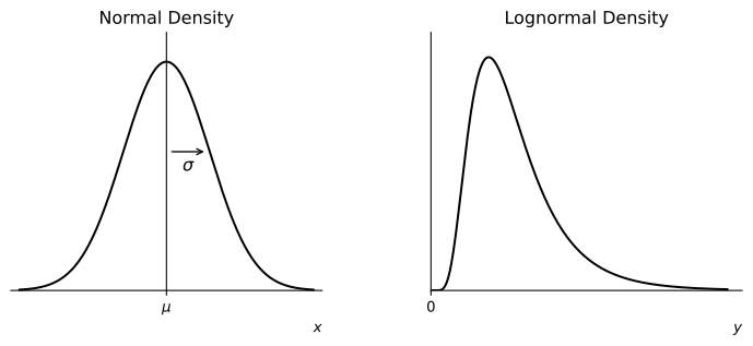
Unlike the normal density, the lognormal density function is not symmetric around its mean. Normally distributed variables can take values in (-\infty, \infty), whereas lognormally distributed variables are always positive.

Computing Probabilities

We can use the fact that the logarithm of a lognormal random variable is normally distributed to compute cumulative probabilities. Specifically, if Y = e^{X} where X \sim \mathcal{N}(\mu, \sigma^{2}), then: \operatorname{P}(Y \leq y) = \mathop{\Phi}\!\left(\frac{\ln(y) - \mu}{\sigma}\right).

Example 5 Let Y = e^{4 + 1.5 Z} where Z \sim \mathcal{N}(0, 1). What is the probability that Y \leq 100? \operatorname{P}(Y \leq 100) = \operatorname{P}(4 + 1.5 Z \leq \ln(100)) = \operatorname{P}\left(Z \leq \tfrac{\ln(100) - 4}{1.5}\right) = \mathop{\Phi}(0.4034) = 0.6567. Therefore, there is a 65.67% chance that Y is less than or equal to 100.

Probability intervals carry over in the same way. Since the exponential function is increasing, the (1 - \alpha) probability interval of Y = e^{\mu + \sigma Z} is [e^{\mu - \sigma z_{\alpha/2}}, e^{\mu + \sigma z_{\alpha/2}}]. It is not symmetric around the median e^{\mu}: the endpoints are the median divided and multiplied by the same factor e^{\sigma z_{\alpha/2}}. For Y = e^{4 + 1.5 Z}, the 95% probability interval is [e^{4 - 1.96 (1.5)}, e^{4 + 1.96 (1.5)}] = [2.89, 1032.71].

Moments

WarningMoments of a Lognormal Distribution

Let Y = e^{\mu + \sigma Z} where Z \sim \mathcal{N}(0, 1). We have that: \begin{aligned} \operatorname{E}(Y) & = e^{\mu + \frac{1}{2} \sigma^{2}} \\ \operatorname{V}(Y) & = e^{2\mu + \sigma^{2}} (e^{\sigma^{2}} - 1) \\ \operatorname{SD}(Y) & = \operatorname{E}(Y) \sqrt{e^{\sigma^{2}} - 1} \end{aligned}

Proof

Completing the square in the exponent, \sigma z - \frac{1}{2} z^{2} = \frac{1}{2} \sigma^{2} - \frac{1}{2} (z - \sigma)^{2}, so \operatorname{E}(Y) = e^{\mu} \int_{-\infty}^{\infty} e^{\sigma z} \frac{e^{-\frac{1}{2} z^{2}}}{\sqrt{2 \pi}} \, dz = e^{\mu + \frac{1}{2} \sigma^{2}} \int_{-\infty}^{\infty} \frac{e^{-\frac{1}{2} (z - \sigma)^{2}}}{\sqrt{2 \pi}} \, dz = e^{\mu + \frac{1}{2} \sigma^{2}}, since the last integrand is the density of a \mathcal{N}(\sigma, 1) random variable. The same calculation with \alpha \mu and \alpha \sigma in place of \mu and \sigma gives the expectation of any power of Y, \operatorname{E}(Y^{\alpha}) = \operatorname{E}\left(e^{\alpha \mu + \alpha \sigma Z}\right) = e^{\alpha \mu + \frac{1}{2} \alpha^{2} \sigma^{2}}. With \alpha = 2, the variance is \operatorname{V}(Y) = \operatorname{E}(Y^{2}) - \operatorname{E}(Y)^{2} = e^{2 \mu + 2 \sigma^{2}} - e^{2 \mu + \sigma^{2}} = e^{2 \mu + \sigma^{2}} (e^{\sigma^{2}} - 1), and taking the square root gives \operatorname{SD}(Y) = \operatorname{E}(Y) \sqrt{e^{\sigma^{2}} - 1}.

Example 6 Let Y = e^{4 + 1.5 Z} where Z \sim \mathcal{N}(0, 1). The expectation and standard deviation of Y are: \begin{aligned} \operatorname{E}(Y) & = e^{4 + 0.5(1.5^{2})} = 168.17 \\ \operatorname{SD}(Y) & = 168.17 \sqrt{e^{1.5^{2}} - 1} = 489.95 \end{aligned}

The Bivariate Normal Distribution

The returns of two assets, or the shocks to a stock price and an interest rate, are usually correlated. The bivariate normal distribution is the standard model for a pair of normal random variables with a given correlation. The simplest way to describe it is by building it from two independent standard normal random variables.

Let Z_{1} and Z_{2} be independent \mathcal{N}(0, 1) random variables and let -1 \leq \rho \leq 1. Define \begin{aligned} X & = \mu_{X} + \sigma_{X} Z_{1}, \\ Y & = \mu_{Y} + \sigma_{Y} \left(\rho Z_{1} + \sqrt{1 - \rho^{2}} \, Z_{2}\right). \end{aligned} \tag{3} We say that (X, Y) has a bivariate normal distribution with means \mu_{X} and \mu_{Y}, standard deviations \sigma_{X} and \sigma_{Y}, and correlation \rho. The random variable X is clearly normal. The random variable Y is also normal, because a linear combination of independent normal random variables is normal, a fact we prove in the notes on generating functions. The term \rho Z_{1} + \sqrt{1 - \rho^{2}} Z_{2} has mean zero and variance \rho^{2} + (1 - \rho^{2}) = 1, so that Y \sim \mathcal{N}(\mu_{Y}, \sigma_{Y}^{2}). Since Z_{1} and Z_{2} are independent, \operatorname{Cov}(X, Y) = \sigma_{X} \sigma_{Y} \operatorname{Cov}(Z_{1}, \rho Z_{1} + \sqrt{1 - \rho^{2}} Z_{2}) = \rho \, \sigma_{X} \sigma_{Y}, and the correlation between X and Y is \rho.

When |\rho| < 1, the pair (X, Y) has the joint density f(x, y) = \frac{1}{2 \pi \sigma_{X} \sigma_{Y} \sqrt{1 - \rho^{2}}} \exp\left(-\frac{1}{2 (1 - \rho^{2})} \left(z_{x}^{2} - 2 \rho z_{x} z_{y} + z_{y}^{2}\right)\right), where z_{x} = (x - \mu_{X}) / \sigma_{X} and z_{y} = (y - \mu_{Y}) / \sigma_{Y} are the standardized values. We will rarely need this formula, because the construction (3) gives the main properties directly. The same construction, with Brownian motions in place of Z_{1} and Z_{2}, is how we will build correlated Brownian motions.

Figure 9: The figure plots 1,000 simulated pairs (X, Y) from bivariate normal distributions with standard normal marginals and correlations \rho = -0.7, 0, and 0.7.

WarningProperties of the Bivariate Normal Distribution

Let (X, Y) have a bivariate normal distribution with parameters \mu_{X}, \mu_{Y}, \sigma_{X}, \sigma_{Y}, and \rho.

1. Linear combinations. For constants a and b, a X + b Y is normally distributed with mean a \mu_{X} + b \mu_{Y} and variance a^{2} \sigma_{X}^{2} + b^{2} \sigma_{Y}^{2} + 2 a b \rho \sigma_{X} \sigma_{Y}.

2. Conditional distribution. Given X = x, Y is normally distributed with \operatorname{E}(Y \mid X = x) = \mu_{Y} + \rho \frac{\sigma_{Y}}{\sigma_{X}} (x - \mu_{X}), \qquad \operatorname{V}(Y \mid X = x) = \sigma_{Y}^{2} (1 - \rho^{2}).

3. Independence. X and Y are independent if and only if \rho = 0.

Proof

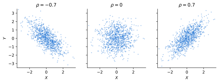
For the first property, (3) shows that a X + b Y is a constant plus a linear combination of the independent normal random variables Z_{1} and Z_{2}, so it is normal. Its mean and variance follow from the formulas for linear combinations in the notes on probability basics.

For the second property, observing X = x is the same as observing Z_{1} = z_{x} = (x - \mu_{X}) / \sigma_{X}. Given this information, Y = \mu_{Y} + \sigma_{Y} \rho z_{x} + \sigma_{Y} \sqrt{1 - \rho^{2}} \, Z_{2}, where Z_{2} is independent of Z_{1} and therefore still has a standard normal distribution. Hence Y is conditionally normal with mean \mu_{Y} + \sigma_{Y} \rho z_{x} and variance \sigma_{Y}^{2} (1 - \rho^{2}).

For the third property, if \rho = 0 then X depends only on Z_{1} and Y depends only on Z_{2}, so they are independent as functions of independent random variables. Conversely, independent random variables are uncorrelated.

The conditional mean is a straight line in x with slope \rho \sigma_{Y} / \sigma_{X} = \operatorname{Cov}(X, Y) / \operatorname{V}(X), the slope of a linear regression of Y on X. For jointly normal random variables the regression line is not just the best linear forecast of Y given X, it is the conditional expectation. Observing X also reduces the variance of Y by the factor 1 - \rho^{2}, regardless of the value observed.

The third property is special to jointly normal random variables. The notes on conditioning and independence show that uncorrelated random variables need not be independent, and the same is true for normal random variables that are not jointly normal. For example, if X \sim \mathcal{N}(0, 1) and S is an independent random sign equal to \pm 1 with probability 1/2, then Y = S X is also standard normal and uncorrelated with X, but |Y| = |X|, so the two are far from independent.

Example 7 The annual returns of two assets are jointly normal with \mu_{A} = 0.08, \sigma_{A} = 0.2, \mu_{B} = 0.05, \sigma_{B} = 0.1, and correlation \rho = 0.3. A portfolio with a weight of 0.6 in asset A and 0.4 in asset B has return R_{p} = 0.6 R_{A} + 0.4 R_{B}, which is normal with mean and variance \begin{aligned} \operatorname{E}(R_{p}) & = 0.6 (0.08) + 0.4 (0.05) = 0.068, \\ \operatorname{V}(R_{p}) & = 0.6^{2} (0.2)^{2} + 0.4^{2} (0.1)^{2} + 2 (0.6)(0.4)(0.3)(0.2)(0.1) = 0.01888. \end{aligned} The standard deviation is \sqrt{0.01888} = 0.1374, and the probability that the portfolio loses money over the year is \operatorname{P}(R_{p} < 0) = \mathop{\Phi}\left(\frac{0 - 0.068}{0.1374}\right) = 0.3103. Because R_{p} is normal, the whole distribution of the portfolio return follows from its mean and variance.

Example 8 Continuing with Example 7, suppose we learn that asset B returned -10\% this year. The conditional distribution of the return of asset A is normal with \begin{aligned} \operatorname{E}(R_{A} \mid R_{B} = -0.10) & = 0.08 + 0.3 \times \frac{0.2}{0.1} (-0.10 - 0.05) = -0.01, \\ \operatorname{SD}(R_{A} \mid R_{B} = -0.10) & = 0.2 \sqrt{1 - 0.3^{2}} = 0.1908. \end{aligned} The slope \rho \sigma_{A} / \sigma_{B} = 0.6 is the beta of asset A with respect to asset B. Learning the return of B moves the forecast of A by 0.6 times the surprise in B, here downward since B fell short of its mean, and reduces the standard deviation of A only slightly, since the correlation is modest.

Heavy Tails

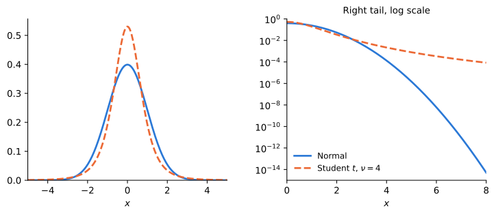
Daily stock returns have far more extreme observations than a normal distribution predicts. Under a normal model a daily move of five standard deviations should occur roughly once every several thousand years, yet stock markets have experienced several such moves in the last few decades. Distributions whose tails decay more slowly than the normal tails are called heavy-tailed, and the Student t distribution is the simplest example.

Let Z \sim \mathcal{N}(0, 1) and let V \sim \text{Gamma}(\nu / 2, 1 / 2) be independent of Z, with \nu > 0. When \nu is an integer, V is chi-squared with \nu degrees of freedom. The random variable T = \frac{Z}{\sqrt{V / \nu}} has a Student t distribution with \nu degrees of freedom. Its density is f(t) = \frac{\Gamma\left(\frac{\nu + 1}{2}\right)}{\sqrt{\nu \pi} \, \Gamma\left(\frac{\nu}{2}\right)} \left(1 + \frac{t^{2}}{\nu}\right)^{-\frac{\nu + 1}{2}}, which is symmetric around zero and bell-shaped, like the normal density. The difference lies in the tails. For large |t| the density decays like the power |t|^{-(\nu + 1)}, whereas the normal density decays like e^{-t^{2} / 2}, which is much faster than any power. Dividing Z by the random scale \sqrt{V / \nu} occasionally produces very large values, which is a useful way to think about returns: they are normal given the level of volatility, but volatility itself is random. As \nu \to \infty, V / \nu \to 1 and the t distribution approaches the standard normal.

Power-law tails have an important consequence for moments. The moment \operatorname{E}(|T|^{k}) is finite only for k < \nu, since for larger k the integrand |t|^{k} f(t) decays too slowly to be integrable. In particular, the t distribution has a finite variance only when \nu > 2, in which case \operatorname{V}(T) = \nu / (\nu - 2). For the same reason, \operatorname{E}(e^{\theta T}) = \infty for every \theta \neq 0, which is one reason we need the characteristic function introduced in the notes on generating functions.

Example 9 To compare a normal and a Student t distribution with the same variance, let X = 0.7071 \, T where T has a t distribution with \nu = 4 degrees of freedom. Since \operatorname{V}(T) = 4 / (4 - 2) = 2, the scaled variable X has unit variance, like a standard normal Z. The probability of a move larger than four standard deviations is \operatorname{P}(|Z| > 4) = 6.33 \times 10^{-5}, \qquad \operatorname{P}(|X| > 4) = 0.0048. The heavy-tailed distribution makes a four standard deviation move about 76 times more likely.

Figure 10: The figure compares a standard normal density with a Student t density with \nu = 4 degrees of freedom, scaled to have unit variance. The right panel shows the right tails on a logarithmic scale.

Summary

The table below collects the distributions studied in these notes.

Distribution	Support	Density f(x)	Mean	Variance
Uniform(a, b)	[a, b]	\frac{1}{b - a}	\frac{a + b}{2}	\frac{(b - a)^{2}}{12}
Exp(\lambda)	[0, \infty)	\lambda e^{-\lambda x}	\frac{1}{\lambda}	\frac{1}{\lambda^{2}}
Gamma(\alpha, \lambda)	(0, \infty)	\frac{\lambda^{\alpha}}{\Gamma(\alpha)} x^{\alpha - 1} e^{-\lambda x}	\frac{\alpha}{\lambda}	\frac{\alpha}{\lambda^{2}}
\mathcal{N}(\mu, \sigma^{2})	\mathbb{R}	\frac{1}{\sqrt{2 \pi \sigma^{2}}} e^{-\frac{(x - \mu)^{2}}{2 \sigma^{2}}}	\mu	\sigma^{2}
Chi-squared(k)	(0, \infty)	\frac{(1/2)^{k/2}}{\Gamma(k/2)} x^{k/2 - 1} e^{-x/2}	k	2 k
Lognormal(\mu, \sigma^{2})	(0, \infty)	\frac{1}{x \sqrt{2 \pi \sigma^{2}}} e^{-\frac{(\ln x - \mu)^{2}}{2 \sigma^{2}}}	e^{\mu + \frac{1}{2} \sigma^{2}}	e^{2 \mu + \sigma^{2}} (e^{\sigma^{2}} - 1)
Student t(\nu)	\mathbb{R}	\propto \left(1 + \frac{x^{2}}{\nu}\right)^{-\frac{\nu + 1}{2}}	0 if \nu > 1	\frac{\nu}{\nu - 2} if \nu > 2