The Index Model

Investment Theory

Lorenzo Naranjo

Fall 2026

Introduction

• Markowitz analysis needs all covariances, and there are many of them.
  • 500 stocks: 125{,}250 variances and covariances from 60{,}000 monthly returns in ten years.
• With more stocks than months, the sample matrix makes some portfolios look riskless.
• With fewer, the noise sits in the portfolios that look least risky, the ones an optimizer picks.
• The cure is structure: returns have a factor structure driven by the market.
  • The index model’s matrix is biased but far more precise.

Who Needs the Covariance Matrix?

• An investor who holds the market needs only the market’s variance.
• Everyone else needs the covariances:
  • to measure a portfolio’s risk: volatility, value at risk, tracking error against a benchmark;
  • to hedge it;
  • to size bets on securities believed to be mispriced.
• The index model answers the first two without the matrix: a portfolio’s risk depends only on its beta and the firm-specific risk of its holdings.
• Sizing bets needs the whole matrix, and that is where structure pays off most.

The Model

• The single index model is a linear regression between the excess returns of a stock and the excess returns of the market portfolio.
• Let’s denote by r_{i} the return of stock i over a given period, and define R_{i} = r_{i} - r_{f} as the excess return over the risk-free asset.
• Similarly, denote by R_{M} the excess return of the market over the risk-free rate.
• The index model postulates R_{i} = \alpha_{i} + \beta_{i} R_{M} + e_{i}, \tag{1} where \operatorname{E}(e_{i}) = 0 and \operatorname{Cov}(R_{M}, e_{i}) = 0.

The Additional Assumption

• \operatorname{E}(e_{i}) = 0 and \operatorname{Cov}(R_{M}, e_{i}) = 0 are not assumptions: with \beta_{i} and \alpha_{i} defined from the moments of returns, they hold by construction, like OLS residuals.
• The one substantive assumption: the market is the only risk that securities share, so \operatorname{Cov}(e_{i}, e_{j}) = 0 for any two different stocks i and j.
  • The residual e_{i} is then firm-specific, or idiosyncratic, risk.
• This is not true in practice.
  • Stocks in the same industry, or with the same style such as value, share shocks the market does not capture.
• The model then understates the risk of bets on what they share: those bets look diversifiable when they are not.

Variance Decomposition

• The assumptions of the single index model imply that the variance of R_{i} can be split into two parts: \begin{aligned} \sigma_{i}^{2} & = \operatorname{V}(\alpha_{i} + \beta_{i} R_{M} + e_{i}) \\ & = \beta_{i}^{2} \operatorname{V}(R_{M}) + \operatorname{V}(e_{i}) + 2 \beta_{i} \operatorname{Cov}(R_{M}, e_{i}) \\ & = \beta_{i}^{2} \sigma_{M}^{2} + \sigma^{2}(e_{i}). \end{aligned} \tag{2}
• The first component of \sigma_{i}^{2} is the systematic variance, which depends on both the beta of the security and the variance of the market.
• The second term of the variance of i is typically computed as the difference between the variance of i and the systematic variance.

Example 1 (Decomposing the Variance) Suppose that you have the following regression for stock A: R_{A} = \alpha_{A} + \beta_{A} R_{M} + e_{A}, where \alpha_{A} = 0.02, \beta_{A} = 1.2, \sigma(e_{A}) = 30\% and \sigma_{M} = 25\%. The variance of A can be computed as follows: \sigma_{A}^{2} = 1.2^{2} \times 0.25^{2} + 0.30^{2} = 0.09 + 0.09 = 0.18. In the previous expression, the systematic and idiosyncratic variances are the same. The standard deviation of A is then \sigma_{A} = \sqrt{0.18} = 42.43\%.

Computing the Beta

• The beta of the model can be estimated from the covariance of R_{i} and R_{M}, and the variance of R_{M}.
• Indeed, we have that \operatorname{Cov}(R_{i}, R_{M}) = \operatorname{Cov}(\beta_{i} R_{M}, R_{M}) + \operatorname{Cov}(e_{i}, R_{M}) = \beta_{i} \operatorname{V}(R_{M}), where we use the fact that \operatorname{Cov}(R_{M}, R_{M}) = \operatorname{V}(R_{M}).
• Thus, in the index model we must have that \beta_{i} = \frac{\operatorname{Cov}(R_{i}, R_{M})}{\operatorname{V}(R_{M})}, \tag{3} just like in the CAPM.

The Security Characteristic Line (SCL)

• The alpha of the security can then be computed as \alpha_{i} = \operatorname{E}(R_{i}) - \beta_{i} \operatorname{E}(R_{M}). \tag{4}
• The line y = \alpha_{i} + \beta_{i} x is called the security characteristic line (SCL) of security i.
  • If we plot this line, \alpha_{i} is the intercept and \beta_{i} is the slope coefficient of the line.

Understanding the Alpha

• A nonzero alpha means the security earns more or less than its market exposure warrants.
• Many independent alphas can add up to a potential arbitrage:
  • Portfolio L holds the positive-alpha securities, portfolio S the negative-alpha ones.
  • With many securities and uncorrelated residuals, their firm-specific risk vanishes.
  • Set both betas to one with the risk-free asset.
• Long L and short S: a zero-cost portfolio with almost no risk and a positive return.

R-Squared

• Following the statistics literature, the proportion of systematic variance to total variance is called the R-squared of security i and can be expressed as \text{R-squared} = \frac{\beta_{i}^{2} \sigma_{M}^{2}}{\sigma_{i}^{2}} = 1 - \frac{\sigma^{2}(e_{i})}{\sigma_{i}^{2}}. \tag{5}
• Therefore, the R-squared can also be expressed as one minus the proportion of idiosyncratic variance to total variance.
• Since the single index model aims to decompose the total variance of a security into two orthogonal components, the R-squared gives us the proportions of this decomposition.

Example 2 (From R-Squared to Volatility) You run the regression R_{B} = \alpha_{B} + \beta_{B} R_{M} + e_{B}. Your regression package reports that \alpha_{B} = -0.01, \beta_{B} = 0.8 and the R-squared is 0.4. If the volatility of the market is 25% per year, the systematic variance is 0.8^{2} \times 0.25^{2} = 0.04. Since 40% of the variance is systematic, we have that \sigma_{B}^{2} = \frac{0.04}{0.4} = 0.10, which implies that \sigma_{B} = \sqrt{0.10} = 31.62\% per year. We also know that 60% of the variance is firm-specific, which means that \sigma^{2}(e_{B}) = 0.6 \times 0.10 = 0.06, so that \sigma(e_{B}) = \sqrt{0.06} = 24.49\% per year.

R-Squared is the Squared Correlation

• Equation (5) can also be expressed in terms of the correlation between R_{i} and R_{M}. \beta_{i} = \frac{\operatorname{Cov}(R_{i}, R_{M})}{\operatorname{V}(R_{M})} = \frac{\sigma_{i} \sigma_{M} \rho_{i, M}}{\sigma_{M}^{2}} = \frac{\sigma_{i} \rho_{i, M}}{\sigma_{M}}, \tag{6} implies \text{R-squared} = \frac{\beta_{i}^{2} \sigma_{M}^{2}}{\sigma_{i}^{2}} = \frac{\frac{\sigma_{i}^{2} \rho_{i, M}^{2}}{\sigma_{M}^{2}} \sigma_{M}^{2}}{\sigma_{i}^{2}} = \rho_{i, M}^{2}. \tag{7}
• The R-squared of a regression of R_{i} on R_{M} is just the square of the correlation between R_{i} and R_{M}.
  • We typically use the Greek letter rho (\rho) for correlation, which corresponds to the Latin letter r.

An Example with Real Data

• Monthly returns of Microsoft, January 2016 to December 2025, from CRSP, dividends included.
• The market is the CRSP value-weighted index of all U.S. stocks.
• The risk-free rate is the one-month Treasury bill, from Kenneth French’s data library.

	Mean (%)	Std. dev. (%)
Microsoft	1.93	5.89
Market	1.08	4.54

• Microsoft’s monthly excess returns were more volatile than the market’s, and so was its average.

Plotting the Data

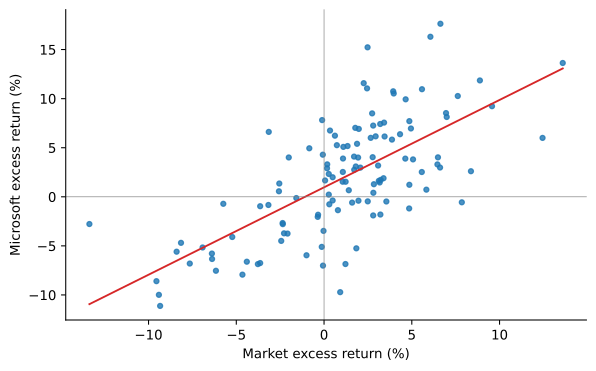
Monthly excess returns of Microsoft against the market, 2016 to 2025, with the security characteristic line.

Regression Results

• We estimate the SCL by ordinary least squares (OLS), with statsmodels.

	Estimate	Std. error	t-statistic	p-value
Alpha	0.0097	0.0039	2.4874	0.0129
Beta	0.8903	0.0873	10.1962	0.0000

• The R-squared is 0.471. Standard errors are robust to heteroskedasticity.

Interpreting the Results

• The intercept is 0.0097, or 0.97% per month, and the beta is 0.8903.
• With a beta a little below one, Microsoft carried a little less systematic risk than the market.
• As a check, the R-squared from the beta and the two volatilities:

\text{R-squared} = \frac{0.8903^{2} \times 4.543^{2}}{5.894^{2}} = 0.471.

More Stocks

Monthly excess returns of Citigroup, BlackRock, Nvidia and Tesla against the market, 2016 to 2025, with their security characteristic lines.

Regression Estimates

	Alpha (%)	p-value	Beta	R-squared	Correlation
C	-0.460	0.439	1.535	0.551	0.742
BLK	-0.126	0.769	1.275	0.651	0.807
NVDA	3.434	0.001	1.801	0.357	0.597
TSLA	1.952	0.171	2.042	0.255	0.505

• Each R-squared is the square of the stock’s correlation with the market.

Analysis

• Tesla has the lowest R-squared, while about 65% of BlackRock’s variance is explained by the market.
• Nvidia and Tesla have high betas: their cash flows are exposed to how the economy does.
• Citigroup also has a high beta, typical of financial firms.
• BlackRock has the lowest beta of the four, still higher than Microsoft’s.
• Nvidia is the only one with an alpha significant at 1%: 3.43% per month.

A Past Alpha Is Not a Forecast

• The four stocks were chosen in 2025, and Nvidia and Tesla are well known precisely because they did spectacularly well.
  • Including them selects on the outcome.
• More generally, a large past alpha is a poor forecast of the next one.
  • Treynor-Black: five-year alphas of the largest stocks say nothing about next year’s.
  • Skill versus Luck: the same holds for mutual funds.
• The estimated alpha is \hat{\alpha}_{i} = \bar{R}_{i} - \hat{\beta}_{i} \bar{R}_{M}: trading on past alphas is trading on past average returns.
  • Can Regression Alphas Beat the CAPM?: a mean-variance investor who does so with the 100 largest stocks loses to the market.

Not All Alphas Are Equal

• Corporate finance teaches that an undervalued firm is a buy: if the shares trade below the value of the cash flows, buy them.
• Mispricing alone is not enough.
  • Buying a stock to earn its alpha also means holding its firm-specific risk e_{i}, and firm-specific risk earns no premium of its own.
  • Nvidia’s alpha is large, but an alpha has to be judged against the firm-specific risk you bear to collect it.
• A large mispricing can be a worse opportunity than a small one.

The Information Ratio

• Scale each alpha by the firm-specific risk that comes with it: \mathit{IR}_{i} = \frac{\alpha_{i}}{\sigma(e_{i})}. \tag{8}
• Stock 1: alpha 2\%, residual volatility 10\%, so \mathit{IR} = 0.2.
• Stock 2: alpha 10\%, five times larger, residual volatility 100\%, so \mathit{IR} = 0.1.
• In the Treynor-Black model, each security’s weight in the active portfolio is proportional to \alpha_{i}/\sigma^{2}(e_{i}): 2 for stock 1, 0.1 for stock 2.
  • The smaller mispricing deserves twenty times the weight.
• Buying more of stock 2 does not help: a bigger position scales its alpha and its risk together and leaves the \mathit{IR} where it was.

Estimating Beta

• An estimated beta is not the true beta. With T monthly observations, \text{SE}(\hat{\beta}_{i}) = \frac{\sigma(e_{i})}{\sigma_{M} \sqrt{T}}.
• Ten years of data give Tesla’s beta a robust standard error of 0.36, BlackRock’s 0.11; the formula, which assumes homoskedastic residuals, gives 0.32 and 0.09.
  • A 95% confidence interval for Tesla’s beta runs from 1.3 to 2.7.
• The highest estimates were pushed up by noise, and the lowest down. True betas also change over time.

Betas Regress toward One

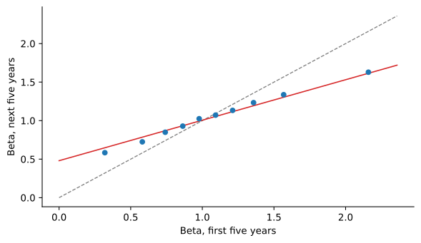
Average beta over five years against the beta over the previous five years, for the 500 largest U.S. stocks with returns in both windows, all windows from 1931 to 2025 pooled and sorted into ten groups.

• \hat{\beta}_{\text{next}} = 0.48 + 0.53 \, \hat{\beta}_{\text{now}}: betas move about halfway back toward the average.

Shrinking Betas

• Vasicek (1973): shrink each estimate toward the cross-sectional mean according to its precision (normal betas and errors), \beta_{i}^{V} = w_{i} \hat{\beta}_{i} + (1 - w_{i}) \bar{\beta}, \qquad w_{i} = \frac{\sigma_{\beta}^{2}}{\sigma_{\beta}^{2} + \text{SE}^{2}(\hat{\beta}_{i})}, where \sigma_{\beta}^{2} is the variance of the estimates minus the average squared standard error.
• Tesla gets a weight of 0.60 and shrinks from 2.04 to 1.64; BlackRock keeps 0.96.
• Commercial data services use one weight for all, the adjusted beta (Blume 1971): \beta_{\text{adj}} = \tfrac{2}{3} \hat{\beta} + \tfrac{1}{3} \times 1.

Noise or Real Change?

• Noise is about 24% of the variance of estimated betas across stocks.
  • Vasicek shrinks about 22% of the way; the data move about halfway.
  • The rest is real change in betas (Blume 1975).
• Squared error against the next estimated beta: OLS 0.254, Vasicek 0.207, adjusted 0.195.
• Current practice (Levi and Welch 2017): one to four years of daily returns, Vasicek, then another 20% to 30% toward the mean.

No Perfect Correlation

• We saw before that if A and B are perfectly correlated, we must have that R_{B} = w R_{A} for some w \neq 0.
  • If this were the case, the covariance between e_{A} and e_{B} is not zero even though they are different assets.
  • More precisely, we have that \operatorname{Cov}(e_{A}, e_{B}) = \operatorname{Cov}(e_{A}, w e_{A}) = w \sigma^{2}(e_{A}) \neq 0, provided that w \neq 0, i.e., you do not invest everything in the risk-free asset.
• In the following, when we talk about two different assets it is implicitly assumed that their excess returns are not perfectly correlated, unless stated otherwise.

Covariance Structure

• The covariance of the excess returns between securities i and j is \operatorname{Cov}(R_{i}, R_{j}) = \operatorname{Cov}(\alpha_{i} + \beta_{i} R_{M} + e_{i}, \alpha_{j} + \beta_{j} R_{M} + e_{j}) = \beta_{i} \beta_{j} \sigma_{M}^{2}. \tag{9}
• The previous expression says that in the single index model, the covariance between any two different securities is given by their exposures to the market and the variance of the market.

Example 3 (Computing a Covariance) Suppose that you have run regressions of excess returns of two securities A and B on the excess returns of the market. You find that \beta_{A} = 1.2 and \beta_{B} = 0.9. If the volatility of the market is 25% per year, then \operatorname{Cov}(R_{A}, R_{B}) = 1.2 \times 0.9 \times 0.25^{2} = 0.0675. If in addition we know that \sigma_{A} = 30\% and \sigma_{B} = 35\%, then we also have \rho_{A, B} = \frac{0.0675}{0.30 \times 0.35} = 0.643.

Correlation Structure

• We can express equation (9) in terms of correlations as \begin{aligned} \rho_{i, j} & = \frac{\beta_{i} \beta_{j} \sigma_{M}^{2}}{\sigma_{i} \sigma_{j}} = \frac{\sigma_{i} \rho_{i, M}}{\sigma_{M}} \, \frac{\sigma_{j} \rho_{j, M}}{\sigma_{M}} \, \frac{\sigma_{M}^{2}}{\sigma_{i} \sigma_{j}} \\ & = \rho_{i, M} \rho_{j, M}. \end{aligned} \tag{10}
• Therefore, in the single-index model, all pairwise correlations between two assets can be computed as the product of their correlations with the market.

The Covariance Matrix

• With the variance decomposition, the covariances give the whole matrix of N securities: \pmb{\Sigma} = \sigma_{M}^{2} \pmb{\beta} \pmb{\beta}^{\top} + \mathbf{D}, where \mathbf{D} is the diagonal matrix of residual variances.
• For 500 stocks: 1{,}001 estimates instead of 125{,}250.
• Biased whenever residuals are correlated, since it sets their covariances to zero, but far more precise than the sample matrix.
  • In Estimation Risk and Shrinkage, minimum-variance portfolios built from it are far less volatile out of sample.

Portfolio Risk Through Betas

• A portfolio with weights w_{i} (the rest in the risk-free asset) has R_{P} = \alpha_{P} + \beta_{P} R_{M} + \sum_{i} w_{i} e_{i}, so \sigma_{P}^{2} = \beta_{P}^{2} \sigma_{M}^{2} + \sum_{i=1}^{N} w_{i}^{2} \sigma^{2}(e_{i}), \qquad \beta_{P} = \sum_{i=1}^{N} w_{i} \beta_{i}. \tag{11}
• 2N + 1 numbers say how risky the portfolio is and how much of that risk is the market’s.
• With active weights w_{i} - w_{i}^{B} in place of w_{i}: the squared tracking error against a benchmark.
• A short position of \beta_{P} in the market removes the first term: hedging leaves only firm-specific risk.

Signal and Noise in Eigenvalues

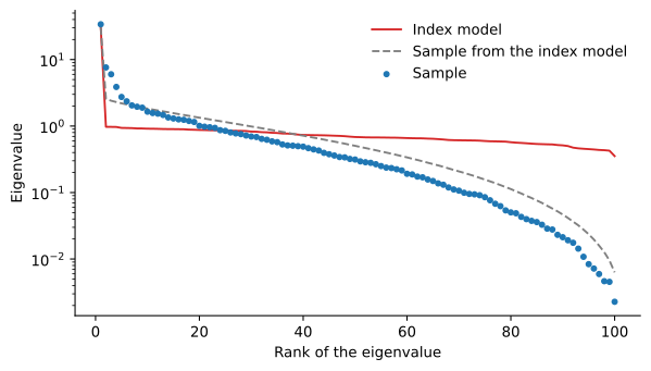
Eigenvalues of the correlation matrix of the 100 largest U.S. stocks, monthly, 2016 to 2025, logarithmic scale.

• Under the index model, every eigenvalue but the first lies between 0.35 and 0.97; 120 months of data spread them from 2.6 to 0.006.

Known Alphas, Estimated Covariances

• With no alphas, hold the market: the matrix matters to an investor with alphas to bet on.
• Truth: the index model plus five residual factors that carry the alphas. The investor knows \pmb{\mu} and estimates \pmb{\Sigma} from 120 months. Best Sharpe ratio 0.74, market 0.38.

Matrix	Investor’s estimate	True value
Sample	1.91	0.30
Index model	1.82	0.63
Five-factor	1.03	0.64

• The index model is wrong but stable, and beats the noisy sample matrix. Its investor still overrates the bets: residual factors look diversifiable.

Beyond a Single Index

• The key assumption, uncorrelated residuals, is only an approximation.
  • Stocks in the same industry share shocks the market does not capture: oil prices, interest rates.
• A model with an index for each common source of risk captures more of the comovement: Beyond the CAPM.
  • Practitioners use multifactor risk models mainly to forecast risk and tracking error: underestimated risk means oversized positions.
• Modern estimators start from the sample matrix and discipline it:
  • shrink it toward the index model (Ledoit and Wolf 2003), or shrink each eigenvalue separately (Ledoit and Wolf 2017).
• The same regression is the standard test of the CAPM: every alpha should be zero (CAPM Anomalies).

References

Blume, Marshall E. 1971. “On the Assessment of Risk.” Journal of Finance 26 (1): 1–10.

Blume, Marshall E. 1975. “Betas and Their Regression Tendencies.” Journal of Finance 30 (3): 785–95.

Ledoit, Olivier, and Michael Wolf. 2003. “Improved Estimation of the Covariance Matrix of Stock Returns with an Application to Portfolio Selection.” Journal of Empirical Finance 10 (5): 603–21.

Ledoit, Olivier, and Michael Wolf. 2017. “Nonlinear Shrinkage of the Covariance Matrix for Portfolio Selection: Markowitz Meets Goldilocks.” Review of Financial Studies 30 (12): 4349–88.

Levi, Yaron, and Ivo Welch. 2017. “Best Practice for Cost-of-Capital Estimates.” Journal of Financial and Quantitative Analysis 52 (2): 427–63.

Vasicek, Oldrich A. 1973. “A Note on Using Cross-Sectional Information in Bayesian Estimation of Security Betas.” Journal of Finance 28 (5): 1233–39.