The Treynor-Black Model

Investment Theory

Lorenzo Naranjo

Fall 2026

Security Analysis and the Market

• A research team can analyze a few dozen stocks at most; the rest are best treated as fairly priced.
• Treynor and Black (1973): hold the market, which needs no forecasts, and add an active portfolio of the securities the analysts believe are mispriced.
• The index model keeps the inputs manageable: \alpha_{i}, \beta_{i} and \sigma^{2}(e_{i}) for each analyzed security, and \operatorname{E}(R_{M}) and \sigma_{M}^{2} for the market.

Model Setup

• We have N risky assets with excess returns following a single-index model R_{i} = \alpha_{i} + \beta_{i} R_{M} + e_{i}, where \operatorname{E}(e_{i}) = 0, \operatorname{Cov}(R_{M}, e_{i}) = 0 and \operatorname{Cov}(e_{i}, e_{j}) = 0 for i \neq j, for all i, j = 1, \ldots, N.
• Suppose we form a portfolio P with the N risky assets and the market portfolio M.
• Denote by w_{i} the weights of the N risky assets and w_{M} the weight in the market portfolio so that \sum_{i = 1}^{N} w_{i} + w_{M} = 1.

The Portfolio’s Alpha

• We can write the excess returns of this portfolio over the risk-free asset as R_{P} = \alpha_{P} + \beta_{P} R_{M} + e_{P}.
  • The portfolio alpha includes the alpha of all the securities except the market that has no alpha.
• Therefore, \alpha_{P} = \sum_{i = 1}^{N} w_{i} \alpha_{i}.
• We will see later that the alpha of the optimal portfolio is positive since its weights are positive for securities with positive alpha, and negative otherwise.

The Portfolio’s Beta

• The beta of this portfolio is a weighted average of the beta of all securities and the beta of the market, which is one.
• Thus, \beta_{P} = \sum_{i = 1}^{N} w_{i} \beta_{i} + w_{M}.

The Portfolio’s Idiosyncratic Risk

• The idiosyncratic risk includes the firm-specific risks of all securities except the market that has no idiosyncratic risk.
• Because the firm-specific risks are uncorrelated with each other, we have that \sigma^{2}(e_{P}) = \sum_{i = 1}^{N} w_{i}^{2} \sigma^{2}(e_{i}).

Portfolio Statistics

• We can compute the portfolio expected return and standard deviation as \operatorname{E}(R_{P}) = \sum_{i = 1}^{N} w_{i} \alpha_{i} + \beta_{P} \operatorname{E}(R_{M}), \tag{1} and \sigma_{P}^{2} = \beta_{P}^{2} \sigma_{M}^{2} + \sum_{i = 1}^{N} w_{i}^{2} \sigma^{2}(e_{i}). \tag{2}

The Idea

• The expected return and variance in (1) and (2) depend on the alphas generated by the active securities and the systematic exposure of the resulting portfolio.
  • This is the essence of the Treynor-Black model.
  • The active part of the portfolio, which might behave like a zero-cost portfolio, generates an alpha but might increase the total risk by adding diversifiable risk.
  • It might also increase the expected return by loading on systematic risk, and therefore increase the systematic risk of the resulting portfolio.

Model Inputs

• Determine a list of securities that you believe are mispriced.
• Use your market research to determine \alpha_{i} for each mispriced security.
  • Remember that \alpha_{i} is positive if you think that the security is undervalued and negative otherwise.
• Run regressions for all securities in your active portfolio and get \beta_{i} and \sigma^{2}(e_{i}) = \sigma_{i}^{2} - \beta_{i}^{2} \sigma_{M}^{2}.
• Obtain an estimate for the market risk-premium \operatorname{E}(R_{M}) = \mu_{M} - r_{f}.
• Compute the variance of market returns \sigma_{M}^{2}.

Solving the Model

• The objective is to find the portfolio weights w_{1}, w_{2}, \ldots, w_{N} and w_{M} that maximize its Sharpe ratio.
• Since \beta_{P} = \sum_{i = 1}^{N} w_{i} \beta_{i} + w_{M}, this is equivalent to finding w_{1}, w_{2}, \ldots, w_{N} and the beta of the final portfolio that maximize the Sharpe ratio of the target portfolio.
• Maximizing the Sharpe ratio is equivalent to minimizing the variance of the portfolio for a given expected return.
  • Only one particular expected return satisfies that the sum of the weights is one.
  • For other targets of the expected return, we would have to borrow or invest the difference at the risk-free rate.

Mathematical Formulation

• If we denote by \mu_{P} a possible target expected return, the minimization problem is as follows: \min_{\{w_{1}, \ldots, w_{N}, \beta_{P}\}} \; \frac{1}{2} \sigma_{P}^{2} \quad \textrm{s.t.} \quad \operatorname{E}(R_{P}) = \mu_{P} - r_{f}.
• If you are interested in how to solve the model see the notes.
  • You need to use some standard constrained optimization calculus techniques, i.e. form a Lagrangian and compute first-order conditions.

The Solution

• Compute \lambda = \frac{1}{\frac{\operatorname{E}(R_{M})}{\sigma^{2}_{M}} + \sum_{i = 1}^{N} \frac{\alpha_{i}}{\sigma^{2}(e_{i})} (1 - \beta_{i})}.
• The portfolio weights are w_{i} = \lambda \frac{\alpha_{i}}{\sigma^{2}(e_{i})}, \qquad w_{M} = 1 - \sum_{i = 1}^{N} w_{i}. \tag{3}
• Weights rise with \alpha_{i} and fall with \sigma^{2}(e_{i}): the quality of the alpha matters.
• Negative alphas get negative weights: those securities are sold short.

The Active Portfolio

• The securities enter in fixed proportions \alpha_{i} / \sigma^{2}(e_{i}), whatever \lambda, so the solution reads in two steps.
• First, the active portfolio A with weights w_{i}^{A} \propto \alpha_{i} / \sigma^{2}(e_{i}), and its \alpha_{A}, \beta_{A} and \sigma^{2}(e_{A}).
• Second, combine A with the market: w_{A}^{0} = \frac{\alpha_{A} / \sigma^{2}(e_{A})}{\operatorname{E}(R_{M}) / \sigma_{M}^{2}}, \qquad w_{A}^{*} = \frac{w_{A}^{0}}{1 + (1 - \beta_{A}) w_{A}^{0}}.
  • w_{A}^{0} is the position if \beta_{A} were one; the adjustment raises it when \beta_{A} > 1, since part of A replaces the market.

Example 1 (An Active Portfolio of Three Stocks) With \operatorname{E}(R_{M}) = 8\% and \sigma_{M} = 20\%:

	Alpha (%)	Beta	Residual vol. (%)	In A (%)	In P (%)
Ashford	3.0	1.2	30.0	49.0	16.1
Brightwater	1.5	0.8	15.0	98.0	32.3
Calder	-2.0	1.0	25.0	-47.1	-15.5
Market		1.0			67.1

A has \alpha_{A} = 3.88\%, \beta_{A} = 0.90 and \sigma(e_{A}) = 23.9\%, so w_{A}^{*} = 0.329 and the Sharpe ratio rises from 0.400 to 0.432.

The Geometry

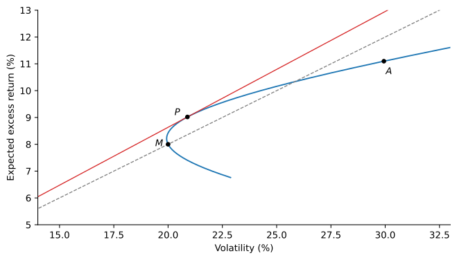
Portfolios combining the active portfolio A with the market M. The optimal portfolio P has the steepest capital allocation line (solid); the dashed line is the market’s.

The Portfolio’s Sharpe Ratio

• We can prove the following relationship between the Sharpe ratio of the optimal portfolio and the market Sharpe ratio, \left( \frac{\operatorname{E}(R_{P})}{\sigma_{P}} \right)^{2} = \sum_{i = 1}^{N} \left(\frac{\alpha_{i}}{\sigma(e_{i})}\right)^{2} + \left( \frac{\operatorname{E}(R_{M})}{\sigma_{M}} \right)^{2}.
• The equation shows that the Sharpe ratio of the optimal portfolio is higher than the Sharpe ratio of the market alone.
  • Each security contributes positively in increasing the Sharpe ratio of the optimal portfolio, regardless of whether the alpha is positive or negative.

The Information Ratio

• For a given security i, the term \alpha_{i} / \sigma(e_{i}) is its information ratio, introduced with the index model, and it measures how good its alpha is.
  • If the volatility of the firm-specific risk is small, then it will be easier to diversify that risk away and hence extract the alpha of the security.
  • Each security contributes to increasing the squared value of the Sharpe ratio of the optimal portfolio by the square of its information ratio.

Many Weak Ideas

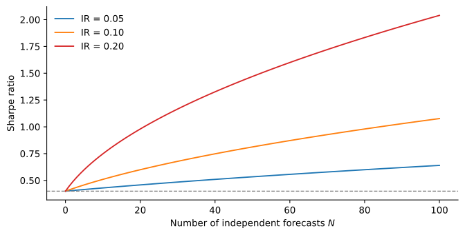
Sharpe ratio with N independent forecasts of equal information ratio, when the market’s Sharpe ratio is 0.40.

• \sqrt{S_{M}^{2} + N \, \mathit{IR}^{2}}: 25 forecasts with \mathit{IR} = 0.1 raise 0.40 to 0.64; with \mathit{IR} = 0.05, only to 0.47.

Adjusting Alpha Forecasts

• Forecasts are noisy: \alpha_{i}^{f} = \alpha_{i} + \varepsilon_{i}. The best estimate of the true alpha shrinks the forecast, \hat{\alpha}_{i} = \frac{\sigma_{\alpha}^{2}}{\sigma_{\alpha}^{2} + \sigma_{\varepsilon}^{2}} \, \alpha_{i}^{f}.
• Estimate the factor from the analyst’s record: the slope of realized alphas on past forecasts.
  • Treynor and Black (1973) propose exactly this regression.
• A forecast shrunk by 0.2 gets a fifth of the weight, and its contribution to the squared Sharpe ratio falls 25-fold.

Historical Alphas as Forecasts

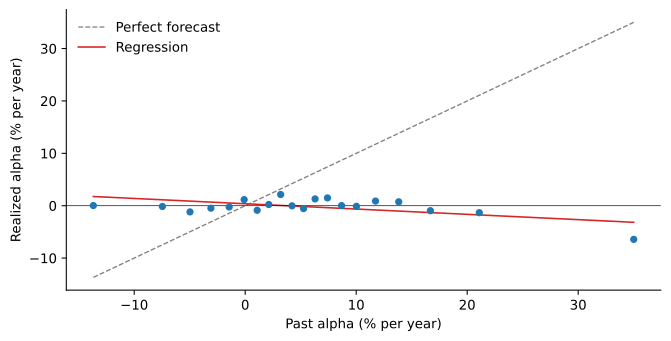
Realized alpha in the next year against the past 60-month alpha, 100 largest U.S. stocks each January, 1932 to 2025, in 20 groups. Annualized.

• The slope of realized on past alphas is -0.10: a large past alpha is mostly luck.

Treynor-Black on Past Alphas

	Mean (%)	Volatility (%)	Sharpe ratio	Worst month (%)
Market	7.57	15.77	0.48	-23.19
Raw forecasts	42.57	172.28	0.25	-385.19

• 1972 to 2025: median active positions 7.5 times wealth, median market weight -3.7.
• In its worst month the portfolio lost more than its value.
• Adjusted forecasts are zero every year, since the slope is never positive: the optimal portfolio is the market.

References

Treynor, Jack L., and Fischer Black. 1973. “How to Use Security Analysis to Improve Portfolio Selection.” Journal of Business 46 (1): 66–86.