Beyond the CAPM
Investment Theory
Fall 2026
From One Factor to Many
- Beta pricing: if a portfolio Q is mean-variance efficient, expected excess returns are proportional to betas with Q.
- The CAPM adds that Q is the market. A multifactor model says instead that Q is a combination of a few factor portfolios.
- Each asset’s excess return follows R_{i,t} = \alpha_{i} + \beta_{i1} F_{1,t} + \cdots + \beta_{iK} F_{K,t} + e_{i,t}, \tag{1} and the model predicts \operatorname{E}(R_{i}) = \beta_{i1} \operatorname{E}(F_{1}) + \cdots + \beta_{iK} \operatorname{E}(F_{K}). \tag{2}
- The test is again whether the alphas are zero.
Why More Than One Factor?
- Intertemporal CAPM (Merton 1973).
- Investors care about changes in investment opportunities, such as future interest rates or expected returns.
- Assets that pay off when opportunities deteriorate are valuable hedges and earn lower expected returns.
- Arbitrage pricing theory (Ross 1976).
- If returns are driven by a few common factors plus firm-specific noise, no arbitrage implies that expected returns are approximately linear in the factor betas.
- Neither theory says which factors to use. In practice, factors have been chosen from the anomalies.
The Three-Factor Model
- Fama and French (1993) built factors from the size and value effects.
- Split stocks into small and big at the NYSE median, and into low, medium and high book-to-market.
- SMB: average of the three small portfolios minus average of the three big ones.
- HML: average of the two high B/M portfolios minus average of the two low ones.
- The model is R_{i,t} = \alpha_{i} + b_{i} MKT_{t} + s_{i} SMB_{t} + h_{i} HML_{t} + e_{i,t}.
- It captures most anomalies known in the mid-1990s, except momentum.
- Carhart (1997) added UMD, past winners minus past losers.
Example 1 (Building SMB and HML) In one month the six size and book-to-market portfolios return S/L 2.0%, S/M 1.5%, S/H 3.0%, B/L 1.0%, B/M 0.8% and B/H 1.6%. Then \begin{aligned} SMB & = \frac{2.0 + 1.5 + 3.0}{3} - \frac{1.0 + 0.8 + 1.6}{3} = 1.03\%, \\ HML & = \frac{3.0 + 1.6}{2} - \frac{2.0 + 1.0}{2} = 0.8\%. \end{aligned} Averaging over small and big makes HML roughly neutral to size.
The Valuation Identity
- Fama and French (2015) start from the dividend discount model: \frac{M_{t}}{B_{t}} = \frac{1}{B_{t}} \sum_{\tau = 1}^{\infty} \frac{\operatorname{E}(Y_{t+\tau} - dB_{t+\tau})}{(1 + r)^{\tau}}, with market value M, book equity B, earnings Y and investment dB.
- Holding everything else fixed, a higher expected return r goes with:
- a higher book-to-market ratio,
- higher expected profitability,
- lower expected investment.
- The identity holds whether prices are rational or not.
Five and Six Factors
- The five-factor model adds RMW (robust minus weak profitability) and CMA (conservative minus aggressive investment): R_{i,t} = \alpha_{i} + b_{i} MKT_{t} + s_{i} SMB_{t} + h_{i} HML_{t} + r_{i} RMW_{t} + c_{i} CMA_{t} + e_{i,t}.
- Main failure: small stocks that invest a lot despite low profitability.
- Striking result: HML becomes redundant, its average return explained by the other four factors.
- The five-factor model also explains low beta and low volatility (Fama and French 2016).
- Adding UMD gives the six-factor model (Fama and French 2018).
Other Models
- q-factor model (Hou et al. 2015), from investment-based asset pricing.
- Firms with high discount rates invest less, and a high expected profitability relative to investment means a high discount rate.
- Factors: market, size (ME), investment (IA) and profitability (ROE).
- Mispricing factors (Stambaugh and Yuan 2017).
- Average rankings across 11 anomalies in two clusters: MGMT (issuance, investment) and PERF (distress, momentum, profitability).
- Behavioral factors (Daniel et al. 2020).
- FIN from issuance and repurchases, PEAD from underreaction to earnings news.
Factor Premia
| Mean (%) | Volatility (%) | Sharpe ratio | t-statistic | |
|---|---|---|---|---|
| MKT | 7.57 | 15.77 | 0.48 | 3.53 |
| SMB | 1.44 | 10.44 | 0.14 | 1.01 |
| HML | 3.48 | 10.70 | 0.33 | 2.39 |
| RMW | 3.42 | 7.99 | 0.43 | 3.15 |
| CMA | 3.11 | 7.07 | 0.44 | 3.23 |
| UMD | 7.08 | 14.99 | 0.47 | 3.47 |
| ME | 2.35 | 10.66 | 0.22 | 1.62 |
| IA | 3.78 | 7.19 | 0.53 | 3.86 |
| ROE | 6.15 | 9.20 | 0.67 | 4.91 |
- Annualized, January 1972 to December 2025; ME, IA and ROE are the q-factors. All premia are positive: ROE has the highest Sharpe ratio, SMB the lowest t-statistic.
Factor Returns over Time
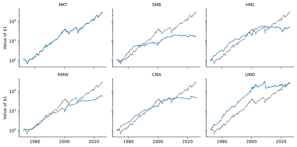
Growth of $1 invested in T-bills plus each Fama-French factor, on a log scale. The gray line is $1 in the market.
Is HML Redundant?
- Most factor correlations are small. The exception is HML and CMA, 0.68: value firms tend to invest conservatively.
- Fama and French warned that the redundancy of HML might be specific to their sample, which ended in 2013.
- Regress HML on MKT, SMB, RMW and CMA:
- July 1963 to December 2013: HML averaged 4.6% a year, alpha -0.1%.
- January 2014 to September 2026: HML averaged -0.8% a year, alpha 0.5% (t = 0.18).
- The value premium disappeared after 2013, and the five-factor model accounts for that too.
Testing a Model with GRS
- Run (1) for each test asset and test whether all alphas are jointly zero: the F-test of Gibbons et al. (1989).
- If the alphas are zero, the factors span the tangency portfolio, and adding the test assets cannot raise the maximum Sharpe ratio.
- The GRS statistic grows with \frac{1 + \theta_{*}^{2}}{1 + \theta_{F}^{2}}, where \theta_{F} is the maximum Sharpe ratio of the factors and \theta_{*} that of the factors and test assets together.
The 25 Size and Book-to-Market Portfolios
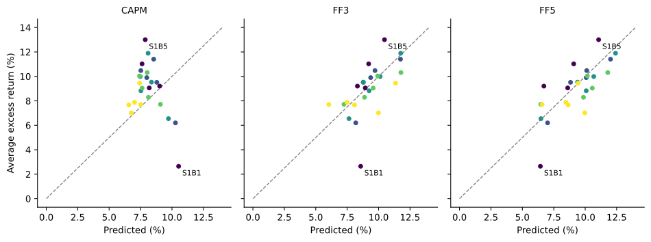
Average annual excess returns of the 25 size and book-to-market portfolios against the returns predicted by three models. Darker points are smaller firms.
GRS Tests
| Mean abs. alpha (%) | Largest abs. t | GRS | p-value | |
|---|---|---|---|---|
| CAPM | 2.17 | 3.41 | 3.68 | < 0.001 |
| FF3 | 1.15 | 4.83 | 3.30 | < 0.001 |
| Carhart | 1.05 | 4.34 | 2.99 | < 0.001 |
| FF5 | 1.10 | 3.75 | 2.92 | < 0.001 |
| FF6 | 1.02 | 3.30 | 2.70 | < 0.001 |
| q-factor | 1.15 | 3.45 | 3.00 | < 0.001 |
- Multifactor models cut the average absolute alpha by more than half, but GRS rejects every model.
- With more than 50 years of data even small alphas are significant; small growth (S1B1) earns far less than any model predicts.
- A model can be rejected and still be useful.
The Anomalies Revisited
| CAPM | FF3 | Carhart | FF5 | FF6 | q-factor | |
|---|---|---|---|---|---|---|
| Size | −0.14 | −0.74 | −0.79 | 0.08 | 0.03 | 1.01 |
| Value | 3.81 | −2.28 | −1.98 | −0.87 | −0.67 | 0.71 |
| Low beta | 6.36 | 4.31 | 1.33 | 0.30 | −1.88 | −1.62 |
| Momentum | 15.72 | 18.71 | 3.51 | 16.15 | 3.15 | 7.59 |
| Reversal | −0.65 | −1.26 | 2.75 | 0.16 | 3.43 | 1.62 |
| Profitability | 6.54 | 5.89 | 5.34 | 0.04 | −0.01 | −0.03 |
| Investment | 5.69 | 2.84 | 1.64 | 0.21 | −0.36 | 0.17 |
| Accruals | 3.56 | 3.40 | 2.69 | 3.51 | 2.91 | 3.10 |
| Low volatility | 14.52 | 11.60 | 8.58 | 5.18 | 3.12 | 3.30 |
- Alphas of the decile spreads, % per year. Bold: |t| > 1.96.
- Significant alphas: CAPM 6, FF3 6, FF5 3, FF6 2.
What the Models Absorb
- The three-factor model overcorrects for value and does nothing for profitability, investment, momentum, accruals or low volatility.
- The five-factor model absorbs profitability, investment and low beta, but leaves momentum as large as under the CAPM.
- Adding UMD brings the momentum alpha down to 3.2% a year.
- The q-factor model has no momentum factor, yet halves the momentum alpha: ROE has a correlation of 0.48 with UMD.
- Accruals keep a significant alpha in almost every model.
Comparing Models by Their Sharpe Ratios
- Every factor is a portfolio that a competing model could use as a test asset.
- So the better model is the one whose factors attain the higher maximum Sharpe ratio (Barillas and Shanken 2018).
- By the Treynor-Black logic, a new factor with alpha \alpha_{k} and residual volatility \sigma(e_{k}) relative to the existing factors raises the maximum squared Sharpe ratio by its squared information ratio: \theta_{\text{new}}^{2} = \theta_{\text{old}}^{2} + \left( \frac{\alpha_{k}}{\sigma(e_{k})} \right)^{2}. \tag{3}
- A factor with a high average return but zero alpha adds nothing.
Maximum Sharpe Ratios
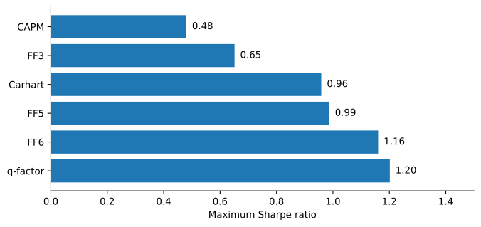
Annualized in-sample maximum Sharpe ratio attainable by combining each model’s factors.
- These are in-sample numbers, chosen with hindsight. They are a fair comparison only because every model gets the same advantage.
Example 2 (Does a New Factor Add Anything?) A model’s factors have a maximum Sharpe ratio of 0.95. Factor A has an alpha of 2.4\% a year relative to them, with residual volatility 8\%, so its information ratio is 0.3 and by (3) the new maximum is \sqrt{0.95^{2} + 0.3^{2}} = 0.996. Factor B averages 4\% a year but has zero alpha, so adding it leaves the maximum at 0.95. This is HML in the five-factor model.
The Factor Zoo
- Hundreds of candidate factors: a “zoo” (Cochrane 2011).
- Are they real?
- How many does a model need?
- Kozak et al. (2020), Lettau and Pelger (2020), Kelly et al. (2019): a handful of well-chosen combinations of characteristics capture most of the information.
- Estimation Risk and Shrinkage takes up these methods.
How Much of the Zoo Do Six Factors Explain?
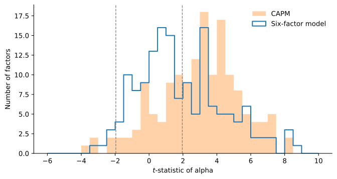
Distribution of the alpha t-statistics of the U.S. factors of Jensen et al. (2023) under the CAPM and the six-factor model. The dashed lines mark \pm 1.96.
- Significant alphas: 72% of 153 factors under the CAPM, 47% under the six-factor model.
Using Factor Models
- Cost of equity: several exposures times their premia, instead of a single beta.
- Risk models: the covariance matrix of many stocks follows from their loadings on a few factors.
- Performance evaluation: a fund that tilts toward small value stocks or past winners has exposures an investor can buy cheaply.
- Only its alpha relative to the factors measures skill.
Example 3 (A Cost of Equity) A five-factor regression gives loadings b = 1.1, s = 0.4, h = 0.3, r = 0.2 and c = -0.1, with premia of 7\%, 2\%, 3.5\%, 3\% and 3\% and a risk-free rate of 4\%. By (2), the expected return is 4\% + 1.1 \times 7\% + 0.4 \times 2\% + 0.3 \times 3.5\% + 0.2 \times 3\% - 0.1 \times 3\% = 13.85\%. With a CAPM beta of 1.15, the CAPM gives 4\% + 1.15 \times 7\% = 12.05\%, almost two points less.