Estimation Risk and Shrinkage

Investment Theory

Lorenzo Naranjo

Fall 2026

Inputs Are Estimated

  • The portfolios of Risky Portfolios, Beta Pricing and Treynor-Black assume known expected returns and covariances.
  • In practice they are estimated, and the estimates are noisy.
  • An optimizer cannot tell estimation error from opportunity.
    • It bets most on the assets whose estimates are most extreme, often the ones most wrong.
  • The remedy: shrinkage, pulling estimates toward a simpler structure that is wrong in detail but less noisy.

Means Are Hard, Variances Are Easy

  • With Y years of data sampled n times (Merton 1980): \text{SE}(\hat{\mu}) = \frac{\sigma}{\sqrt{Y}} \qquad \text{SE}(\hat{\sigma}) \approx \frac{\sigma}{\sqrt{2 n}}.
  • The precision of a mean depends only on the calendar length of the sample; volatility improves with frequency.
  • The U.S. market since 1926: premium 8.3%, volatility 18.4%.
    • Standard error of the premium after 100 years: 1.84%; after 10 years: 5.8%.
    • Standard error of the volatility from 10 years of months: 1.2%.

The Plug-In Portfolio

  • Replace \pmb{\mu} and \pmb{\Sigma} in the tangency weights \pmb{\Sigma}^{-1} \pmb{\mu} with sample estimates.
  • In sample it has the highest Sharpe ratio by construction: it fits the noise.
  • With zero true premia, the in-sample squared monthly Sharpe ratio averages N / T.
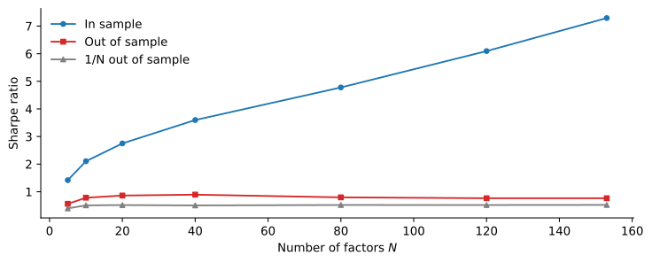
The in-sample Sharpe ratio rises from about 1.4 with 5 factors to about 7.3 with 153. The out-of-sample Sharpe ratio rises from about 0.56 to about 0.89 at 40 factors and declines to about 0.76. The equally weighted portfolio stays near 0.5.

Sharpe ratio of the plug-in portfolio of N JKP factors, estimated 1972 to 1998, in sample and 1999 to 2025, with 1/N.

How Hard Is 1/N to Beat?

  • DeMiguel et al. (2009): 14 models on 7 data sets, none consistently better than 1/N out of sample.
    • The plug-in needs about 3,000 months of data to beat 1/N with 25 assets, 6,000 with 50.
  • Kan and Zhou (2007): with estimation risk, combine the sample tangency with the sample minimum-variance portfolio, which needs no means.
  • Among the JKP factors, with large premia, the plug-in still beats 1/N out of sample: 0.76 against 0.50.
    • Out of sample only for the estimation: many factors were discovered after 1998, and returns are before trading costs.

Shrinking the Covariance Matrix

  • The minimum-variance portfolio isolates the covariance matrix. Three remedies:
  • Structure: the single-index matrix \sigma_{M}^{2} \pmb{\beta} \pmb{\beta}^{\top} + \mathbf{D}, 2N + 1 parameters.
  • Shrinkage (Ledoit and Wolf 2004): \hat{\pmb{\Sigma}}_{\delta} = \delta \pmb{\Sigma}_{\text{CC}} + (1 - \delta) \hat{\pmb{\Sigma}}, \qquad 0 \leq \delta \leq 1, toward the constant-correlation matrix \pmb{\Sigma}_{\text{CC}}, from the sample matrix \hat{\pmb{\Sigma}}, with \delta chosen to minimize expected error.
  • No short sales (Jagannathan and Ma 2003): equivalent to shrinking the largest covariances.

Minimum Variance out of Sample

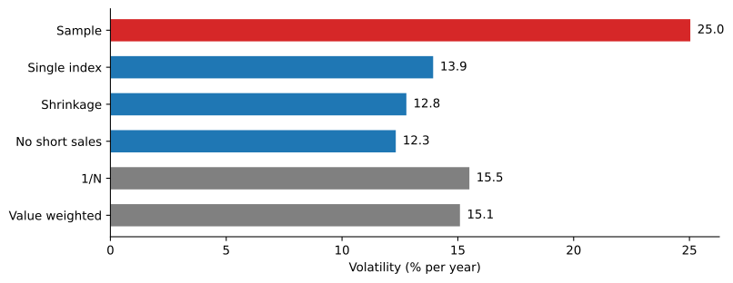
Horizontal bars. The sample covariance matrix gives about 25 percent, the single-index matrix about 14, shrinkage about 13, the sample matrix with no short sales about 12, the equally weighted portfolio about 15.5 and the value-weighted portfolio about 15 percent.

Volatility of minimum-variance portfolios of the 100 largest U.S. stocks, re-estimated each January from 120 months, 1972 to 2025.

  • Average shrinkage intensity: 0.50. For covariances, disciplined estimation pays reliably; for means, only when premia are large.

Black-Litterman

  • Mean-variance optimizers fed with raw forecasts produce extreme portfolios (Black and Litterman 1992).
  • Start from the premiums that make the market optimal, \pmb{\pi} = A \pmb{\Sigma} \mathbf{w}_{M}: the CAPM.
  • A view: portfolio \mathbf{p} earns q, with uncertainty \omega. Then \begin{aligned} \pmb{\mu}_{\text{BL}} & = \pmb{\pi} + \tau \pmb{\Sigma} \mathbf{p} \, \frac{q - \mathbf{p}^{\top} \pmb{\pi}}{\tau \mathbf{p}^{\top} \pmb{\Sigma} \mathbf{p} + \omega}, \\ \mathbf{w}_{\text{BL}} & = \mathbf{w}_{M} + \mathbf{p} \, \frac{\tau (q - \mathbf{p}^{\top} \pmb{\pi})}{A (\tau \mathbf{p}^{\top} \pmb{\Sigma} \mathbf{p} + \omega)}. \end{aligned}
  • The market plus a position in the view portfolio, as in Treynor-Black.

Example 1 (A Relative View) Two assets with volatilities 20% and 15%, correlation 0.5, market weights 60% and 40%, and A = 2.5: equilibrium premiums are 7.5% and 4.5%. An investor expects a 5% spread instead of 3%, as uncertain as the prior, with \tau = 0.05. The posterior premiums are 8.27% and 4.27%, a 4% spread, and the weights become 72.3% and 27.7%.

Ridge and Principal Components

  • In principal components, the tangency portfolio is \pmb{\Sigma}^{-1} \pmb{\mu} = \sum_{j=1}^{N} \mathbf{v}_{j} \, \frac{\mathbf{v}_{j}^{\top} \pmb{\mu}}{\lambda_{j}}: low-variance components get the largest weights, and their estimated means are mostly noise.
  • Kozak et al. (2020): a low-variance component should not have a high Sharpe ratio, or it would be a near-arbitrage.
  • This prior gives the ridge portfolio: \mathbf{w}_{\gamma} = (\hat{\pmb{\Sigma}} + \gamma \mathbf{I})^{-1} \hat{\pmb{\mu}} = \sum_{j=1}^{N} \mathbf{v}_{j} \, \frac{\mathbf{v}_{j}^{\top} \hat{\pmb{\mu}}}{\lambda_{j} + \gamma}.

Shrinkage Trades Fit for Performance

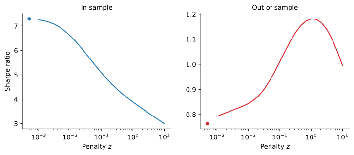
Two panels. In sample, the Sharpe ratio falls from about 7.3 to about 3 as the penalty rises. Out of sample, it rises from about 0.76 to a peak near 1.2 at z equal to 1 and declines to about 1.0 at z equal to 10.

Sharpe ratio of the ridge portfolio of all JKP factors, estimated 1972 to 1998, against the penalty z as a multiple of the average eigenvalue. The points at the left are the plug-in portfolio.

  • Out of sample: 0.76 for the plug-in, 1.18 at z = 1.
    • That z is picked with hindsight, but every z from 0.1 to 10 earns at least 0.99.
    • Choosing z from past data costs little with the full menu, but can fail with only the factors known at the time.

How Many Factors?

  • Kozak et al. (2020): a few characteristic factors cannot summarize the cross-section, but a few principal components can.
  • Lettau and Pelger (2020): PCA with a penalty on pricing errors finds five factors with economic meaning.
  • Kelly et al. (2019): five latent factors with characteristic-based loadings beat existing models.
  • Feng et al. (2020): most new factors are redundant, though a few are not.
  • A few well-chosen combinations beat a short list of anomaly factors. How few is unsettled: five principal components earn about 1.1, against 1.9 for ridge.

The Virtue of Complexity

  • With N > T, many portfolios fit the sample perfectly; the ridgeless portfolio is the one with the smallest weights.
  • It does poorly near N = T and recovers as N grows: “double descent” (Hastie et al. 2022).
  • Kelly et al. (2024): market timing with up to 10,000 parameters from 12 months of data.
    • Out-of-sample Sharpe ratio gains up to about 0.47, with negative R^{2}.
  • Didisheim et al. (2023): SDFs with more factors than observations beat simpler ones.

Complexity in the Factor Zoo

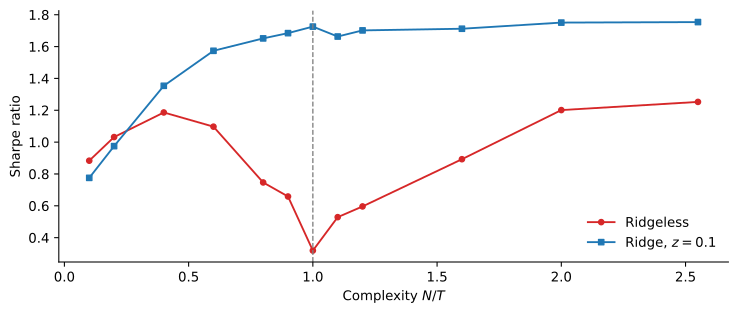
The ridgeless Sharpe ratio rises from about 0.9 to about 1.2 at a complexity of 0.4, falls to about 0.3 at a complexity of 1, marked by a dashed line, and recovers to about 1.25 at 2.5. The ridge Sharpe ratio rises from about 0.8 to about 1.7 at a complexity of 1 and stays between 1.65 and 1.75.

Out-of-sample Sharpe ratio of ridgeless and ridge (z = 0.1) portfolios of N JKP factors, re-estimated monthly from 60 months, against N / T.

  • Ridgeless: 0.32 near N = T, 1.25 with all factors, barely above the best with N < T; ridge: 1.75.

A Debated Virtue

  • Nagel (2025): with 12 months of data, the forecast is a weighted average of recent returns, a volatility-timed momentum strategy.
    • On returns that reverse, the method builds the same strategy and loses money.
  • Kelly and Malamud (2025): placebo predictors with the same persistence produce almost no predictability, and the patterns appear with long samples too.
  • The debate is about learning from very short samples; a large shrunk model can beat a small misspecified one.
  • Our factor test sides with neither: without shrinkage, complexity barely pays; with it, parameters beyond N = T help little.
  • The protection against overfitting is the shrinkage, not a small model.

Takeaways

  • Means are estimated far less precisely than covariances.
  • The plug-in portfolio fits noise; 1/N is a demanding benchmark.
  • Shrinking the covariance matrix, by structure, shrinkage or no short sales, cuts out-of-sample risk sharply.
  • Black-Litterman and ridge shrink expected returns toward the market or toward low Sharpe ratios for low-variance components.
  • Complexity helps only through the shrinkage that comes with it.

References

Black, Fischer, and Robert Litterman. 1992. “Global Portfolio Optimization.” Financial Analysts Journal 48 (5): 28–43.
DeMiguel, Victor, Lorenzo Garlappi, and Raman Uppal. 2009. “Optimal Versus Naive Diversification: How Inefficient Is the 1/N Portfolio Strategy?” Review of Financial Studies 22 (5): 1915–53.
Didisheim, Antoine, Shikun Barry Ke, Bryan T. Kelly, and Semyon Malamud. 2023. Complexity in Factor Pricing Models. Working Paper No. 31689. National Bureau of Economic Research.
Feng, Guanhao, Stefano Giglio, and Dacheng Xiu. 2020. “Taming the Factor Zoo: A Test of New Factors.” Journal of Finance 75 (3): 1327–70.
Hastie, Trevor, Andrea Montanari, Saharon Rosset, and Ryan J. Tibshirani. 2022. “Surprises in High-Dimensional Ridgeless Least Squares Interpolation.” The Annals of Statistics 50 (2): 949–86.
Jagannathan, Ravi, and Tongshu Ma. 2003. “Risk Reduction in Large Portfolios: Why Imposing the Wrong Constraints Helps.” Journal of Finance 58 (4): 1651–83.
Kan, Raymond, and Guofu Zhou. 2007. “Optimal Portfolio Choice with Parameter Uncertainty.” Journal of Financial and Quantitative Analysis 42 (3): 621–56.
Kelly, Bryan T., Seth Pruitt, and Yinan Su. 2019. “Characteristics Are Covariances: A Unified Model of Risk and Return.” Journal of Financial Economics 134 (3): 501–24.
Kelly, Bryan, and Semyon Malamud. 2025. Understanding the Virtue of Complexity. Working Paper No. 5346842. SSRN.
Kelly, Bryan, Semyon Malamud, and Kangying Zhou. 2024. “The Virtue of Complexity in Return Prediction.” The Journal of Finance 79 (1): 459–503.
Kozak, Serhiy, Stefan Nagel, and Shrihari Santosh. 2020. “Shrinking the Cross-Section.” Journal of Financial Economics 135 (2): 271–92.
Ledoit, Olivier, and Michael Wolf. 2004. “Honey, i Shrunk the Sample Covariance Matrix.” Journal of Portfolio Management 30 (4): 110–19.
Lettau, Martin, and Markus Pelger. 2020. “Factors That Fit the Time Series and Cross-Section of Stock Returns.” Review of Financial Studies 33 (5): 2274–325.
Merton, Robert C. 1980. “On Estimating the Expected Return on the Market: An Exploratory Investigation.” Journal of Financial Economics 8 (4): 323–61.
Nagel, Stefan. 2025. Seemingly Virtuous Complexity in Return Prediction. Working Paper No. 34104. National Bureau of Economic Research.