Portfolios of Risky Assets
Investment Theory
Fall 2026
A Portfolio of Two Risky Assets
- Suppose we have two risky assets A and B. The return of a portfolio P in which we invest 1 - w in A and w in B is r_{P} = (1 - w) r_{A} + w r_{B}. \tag{1}
- The expected return of the portfolio is \mu_{P} = (1 - w) \mu_{A} + w \mu_{B}, \tag{2} whereas its variance can be computed as \begin{aligned} \sigma_{P}^{2} & = \operatorname{V}((1 - w) r_{A} + w r_{B}) \\ & = (1 - w)^{2} \sigma_{A}^{2} + w^{2} \sigma_{B}^{2} + 2 w (1 - w) \sigma_{A, B}. \end{aligned} \tag{3}
- Here \sigma_{A, B} denotes the covariance of returns between A and B.
Example 1 (A Portfolio with Two Risky Assets) Consider two risky assets A and B for which you have the following information.
| Asset | Expected Return | Standard Deviation |
|---|---|---|
| A | 10% | 20% |
| B | 15% | 35% |
The correlation between the assets returns is 0.4. If you invest 40% in A and 60% in B, your portfolio will have an expected return of \mu = 0.4 \times 0.10 + 0.6 \times 0.15 = 13.0\%. Since the covariance of returns is \sigma_{AB} = 0.20 \times 0.35 \times 0.4 = 0.028, the standard deviation of the portfolio returns is \sigma = \sqrt{0.4^{2} \times 0.20^{2} + 0.6^{2} \times 0.35^{2} + 2 \times 0.4 \times 0.6 \times 0.028} = 25.29\%.
Short-Selling a Stock
- In financial markets, it is possible to borrow an asset and then sell it.
- We call this transaction short-selling the asset.
- Typically, there is no specific date when the asset must be paid back, but must be paid back as soon as the lender requires it.
- In this class, we assume that short-selling is allowed.
- Short selling implies that w can be greater than one, in which case we borrow A to overinvest in B, or less than zero, in which case we borrow B to overinvest in A.
The Investment Opportunity Set
- The investment opportunity set generated by the two risky assets is an hyperbola.

Figure 1: The figure shows the investment opportunity set generated by two risky assets A and B.
The Minimum Variance Portfolio (MVP)
- As shown in the previous plot, there is a portfolio that has the minimum variance among all portfolios between A and B.
- To find its composition, we can use standard optimization techniques: \begin{aligned} \frac{d}{dw} \sigma_{P}^{2} & = \frac{d}{dw} (1 - w)^{2} \sigma_{A}^{2} + w^{2} \sigma_{B}^{2} + 2 w (1 - w) \sigma_{A, B} \\ & = - 2 (1 - w) \sigma_{A}^{2} + 2 w \sigma_{B}^{2} + 2 (1 - 2 w) \sigma_{A, B} = 0. \end{aligned} \tag{4}
- Thus, - (1 - w) \sigma_{A}^{2} + w \sigma_{B}^{2} + (1 - 2 w) \sigma_{A, B} = 0. or w_{MV} = \frac{\sigma_{A}^{2} - \sigma_{A, B}}{\sigma_{A}^{2} + \sigma_{B}^{2} - 2 \sigma_{A, B}}. \tag{5}
Property 1 (The Minimum Variance Portfolio) Given two risky assets A and B, there is a portfolio that has the minimum variance among all possible portfolios that can be built with A and B. The weights of the minimum variance portfolio are given by \begin{aligned} w_{A} & = \frac{\sigma_{B}^{2} - \sigma_{AB}}{\sigma_{A}^{2} + \sigma_{B}^{2} - 2 \sigma_{AB}}, \\ w_{B} & = \frac{\sigma_{A}^{2} - \sigma_{AB}}{\sigma_{A}^{2} + \sigma_{B}^{2} - 2 \sigma_{AB}}. \end{aligned} In the previous expression, \sigma_{A} and \sigma_{B} denote the standard deviation or volatility of returns. The term \sigma_{AB} denotes the covariance of A and B and is equal to \sigma_{AB} = \sigma_{A} \sigma_{B} \rho_{AB}, where \rho_{AB} is the correlation between the returns of A and B.
Example 2 (Minimum Variance Portfolio) Using the data of Example 1, we find that the weights of the minimum variance portfolio are given by \begin{aligned} w_{A} & = \frac{0.35^{2} - 0.028}{0.20^{2} + 0.35^{2} - 2 \times 0.028} = 88.73\% \\ w_{B} & = \frac{0.20^{2} - 0.028}{0.20^{2} + 0.35^{2} - 2 \times 0.028} = 11.27\% \end{aligned} Thus, the expected return and volatility of the the minimum variance portfolio are \begin{aligned} \mu & = 0.8873 \times 0.10 + 0.1127 \times 0.15 = 10.56\%, \\ \sigma & = \sqrt{0.8873^{2} \times 0.20^{2} + 0.1127^{2} \times 0.35^{2} + 2 \times 0.8873 \times 0.1127 \times 0.028} \\ & = 19.66\%. \end{aligned}
Location of the MVP
- The MVP is the point farthest to the left of the investment opportunity set.

Figure 2: The figure shows the minimum variance portfolio obtained from combining two risky assets.
An Equally-Weighted Portfolio
- Say that we have N securities and we invest the same amount in each, so the return of this portfolio that we call P is r_{P} = \frac{1}{N} \sum_{i = 1}^{N} r_{i}.
- The variance of P is given by \sigma_{P}^{2} = \frac{1}{N^{2}} \sum_{i = 1}^{N} \sum_{j = 1}^{N} \operatorname{Cov}(r_{i}, r_{j}). \tag{6}
Average Variance and Covariance
- The average variance of the securities is \text{Avg. Variance} = \frac{1}{N} \sum_{i = 1}^{N} \operatorname{V}(r_{i})
- The average covariance of the securities is \text{Avg. Covariance} = \frac{1}{N (N - 1)} \sum_{i = 1}^{N} \sum_{\substack{j = 1 \\ i \neq j}}^{N} \operatorname{Cov}(r_{i}, r_{j})
- We can write (6) as \sigma_{P}^{2} = \frac{1}{N} (\text{Average Variance}) + \frac{N - 1}{N} (\text{Average Covariance}). \tag{7}
Understanding Diversification
- As N increases in (7), we have that \sigma_{P}^{2} \xrightarrow[N \rightarrow \infty]{} \text{Average Covariance}.
- The average variance disappears: this is the part of the risk that can be diversified away.
- What remains is the average covariance, which sets a floor on how much risk diversification can remove.
- The 2008 financial crisis illustrated this limit.
- Correlations among mortgage-related assets that had appeared only loosely related rose sharply, so portfolios that seemed well diversified suffered simultaneous losses.
Many Risky Assets
A Portfolio of Many Risky Assets
- With N risky assets, collect returns and weights into vectors \mathbf{r} = (r_{1}, \ldots, r_{N})^{\top} and \pmb{w} = (w_{1}, \ldots, w_{N})^{\top}.
- The weights can be any real numbers, but they must add up to one: \pmb{w}^{\top} \mathbf{1} = 1. \tag{8}
- The portfolio return is the linear combination r_{P} = \pmb{w}^{\top} \mathbf{r} = \sum_{i = 1}^{N} w_{i} r_{i}. \tag{9}
Mean and Variance in Matrix Form
- Let \pmb{\mu} = (\mu_{1}, \ldots, \mu_{N})^{\top} and let \pmb{\Sigma} be the covariance matrix, with entries \sigma_{ij} = \operatorname{Cov}(r_{i}, r_{j}).
- Then \mu_{P} = \pmb{w}^{\top} \pmb{\mu}, \qquad \sigma_{P}^{2} = \pmb{w}^{\top} \pmb{\Sigma} \pmb{w} = \sum_{i = 1}^{N} \sum_{j = 1}^{N} w_{i} w_{j} \sigma_{ij}. \tag{10}
- For two portfolios P and Q, \operatorname{Cov}(r_{P}, r_{Q}) = \pmb{w}_{P}^{\top} \pmb{\Sigma} \pmb{w}_{Q}. \tag{11}
- With N = 2 these formulas collapse to (2) and (3).
Example 3 (A Portfolio of Three Risky Assets) Three assets have expected returns of 8%, 12%, and 15%, standard deviations of 15%, 20%, and 25%, and correlations \rho_{AB} = 0.3, \rho_{AC} = 0.1, and \rho_{BC} = 0.4, so \pmb{\Sigma} = \begin{pmatrix} 0.0225 & 0.0090 & 0.00375 \\ 0.0090 & 0.0400 & 0.0200 \\ 0.00375 & 0.0200 & 0.0625 \end{pmatrix}. With \pmb{w} = (0.3, 0.3, 0.4)^{\top}, (10) gives \mu_{P} = 12.0\% and \sigma_{P}^{2} = 0.0229, so \sigma_{P} = 15.15\%.
The Investment Opportunity Set with Many Assets
- With N \geq 3 assets, many portfolios share the same expected return but differ in variance.
- The investment opportunity set is a filled region, not a curve.
- Its left boundary is the minimum-variance frontier: for each target return m, \min_{\pmb{w}} \; \pmb{w}^{\top} \pmb{\Sigma} \pmb{w} \quad \text{subject to} \quad \pmb{w}^{\top} \mathbf{1} = 1 \quad \text{and} \quad \pmb{w}^{\top} \pmb{\mu} = m.
The Minimum-Variance Frontier
- The solution gives \sigma_{P}^{2}(m) = \frac{C m^{2} - 2 A m + B}{D}, \tag{12} where A = \pmb{\mu}^{\top} \pmb{\Sigma}^{-1} \mathbf{1}, B = \pmb{\mu}^{\top} \pmb{\Sigma}^{-1} \pmb{\mu}, C = \mathbf{1}^{\top} \pmb{\Sigma}^{-1} \mathbf{1}, and D = BC - A^{2}.
- This is a parabola in (\sigma_{P}^{2}, \mu_{P})-space, hence a hyperbola in (\sigma_{P}, \mu_{P})-space, as with two assets.
- Its minimum, at m = A/C with \sigma_{P}^{2} = 1/C, is the minimum-variance portfolio.
The Frontier with Three Assets
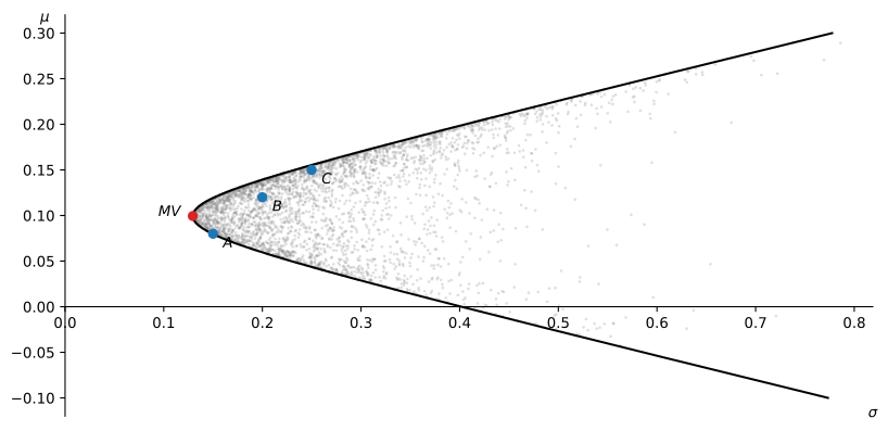
Figure 3: Portfolios of three risky assets fill a region bounded on the left by the minimum-variance frontier.
The MVP with Many Assets
- Minimize \pmb{w}^{\top} \pmb{\Sigma} \pmb{w} subject to \pmb{w}^{\top} \mathbf{1} = 1 with the Lagrangian L(\pmb{w}, \lambda) = \pmb{w}^{\top} \pmb{\Sigma} \pmb{w} - 2 \lambda \left( \pmb{w}^{\top} \mathbf{1} - 1 \right).
- The first-order condition gives \pmb{w} = \lambda \pmb{\Sigma}^{-1} \mathbf{1}.
- \pmb{\Sigma}^{-1} exists because \pmb{\Sigma} is positive definite: \pmb{w}^{\top} \pmb{\Sigma} \pmb{w} is a portfolio variance, positive as long as no combination of the assets is riskless.
- The budget constraint pins down \lambda = 1 / (\mathbf{1}^{\top} \pmb{\Sigma}^{-1} \mathbf{1}).
Property 2 (The Minimum-Variance Portfolio with Many Assets) Given N risky assets with covariance matrix \pmb{\Sigma}, the minimum-variance portfolio has weights \pmb{w}_{MV} = \frac{\pmb{\Sigma}^{-1} \mathbf{1}}{\mathbf{1}^{\top} \pmb{\Sigma}^{-1} \mathbf{1}} \tag{13} and variance \sigma_{MV}^{2} = \frac{1}{\mathbf{1}^{\top} \pmb{\Sigma}^{-1} \mathbf{1}}. \tag{14} With N = 2, the weights reduce to those in Property 1.
Properties of the Minimum Variance Portfolio
- For any portfolio P with \pmb{w}_{P}^{\top} \mathbf{1} = 1, (11) and \pmb{w}_{MV} = \lambda \pmb{\Sigma}^{-1} \mathbf{1} give \operatorname{Cov}(r_{P}, r_{MV}) = \pmb{w}_{P}^{\top} \pmb{\Sigma} \left( \lambda \pmb{\Sigma}^{-1} \mathbf{1} \right) = \lambda = \sigma_{MV}^{2}.
- The covariance of the MVP with any other portfolio is always the same and equal to its own variance!
- The correlation of the MVP with any other portfolio is always positive.
Example 5 (Computing a Correlation with the MVP) Consider an investment opportunity set where the MVP has a standard deviation of returns of 20%. An asset A has a standard deviation of returns equal to 30%. Thus, \sigma_{A} \sigma_{MV} \rho_{A, MV} = \sigma_{A, MV} = \sigma_{MV}^{2}, or \rho_{A, MV} = \frac{\sigma_{MV}}{\sigma_{A}} = \frac{2}{3}.
Why Practitioners Like the MVP
- The MVP weights depend only on variances and covariances, which can be estimated with good precision.
- Every other portfolio in the opportunity set also needs expected returns, which are much harder to estimate.
- Forbidding short sales makes the estimated MVP more robust.
- With fewer months of returns than stocks, the sample covariance matrix is singular; ruling out short sales removes the long-short positions the data cannot pin down, so the problem has a solution.
- When the sample matrix is invertible, the constraint is equivalent to shrinking the largest covariance estimates (Jagannathan and Ma, 2003).
- Once short sales are ruled out, the sample covariance matrix performs as well as factor models, shrinkage estimators, and daily data.