Beta Pricing

Investment Theory

Lorenzo Naranjo

Fall 2026

Adding a Risk-Free Asset

• Adding a risk-free asset allows us to generate a CAL for each risky portfolio in our original investment opportunity set.

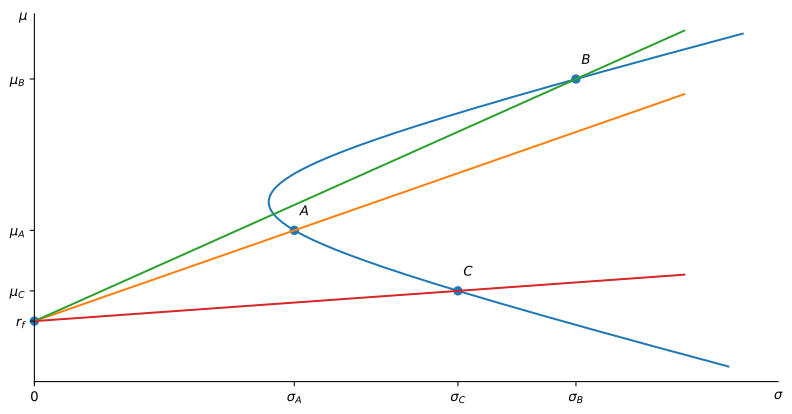
Figure 1: The figure shows the capital allocation lines of portfolios A, B, and C that are members of the same investment opportunity set of risky assets.

The Tangency Portfolio

• There is one portfolio Q that achieves the highest Sharpe ratio.

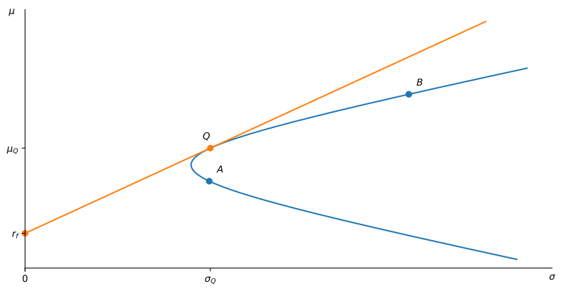
Figure 2: The figure shows the capital allocation line of the tangency portfolio.

The Efficient Frontier

• Investors who prefer portfolios with the highest Sharpe ratio will choose a portfolio located in the CAL of the tangency portfolio.
• We call this CAL the efficient frontier.
• All portfolios in this CAL are efficient portfolios since they all have the highest Sharpe ratio.
  • Any two portfolios in this line are enough to generate all the other efficient portfolios.
• Any other portfolios in this economy will have lower Sharpe ratios than the tangency portfolio.
  • To determine if a portfolio is efficient or not, just compute its Sharpe ratio and compare it to the Sharpe ratio of an efficient portfolio.

The New Investment Opportunity Set

• Shorting Q to invest more than 100% in the risk-free asset traces a mirror-image line through r_{f}.
• Together with the CAL of Q, it encloses the hyperbola: once the risk-free asset is available, the opportunity set is a triangle.

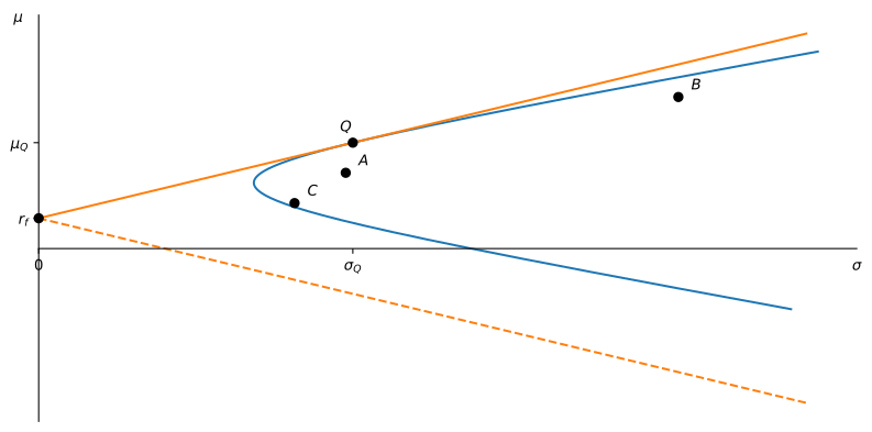
Figure 3: The CAL of Q and its mirror image, obtained by shorting Q, enclose the risky-asset hyperbola.

What the Triangle Means

• Every efficient portfolio combines the risk-free asset with Q.
• A mean-variance investor’s problem collapses to capital allocation: how much to put in Q and how much in the risk-free asset.
• Only mean-variance preferences make an investor maximize the Sharpe ratio.
  • Investors with other preferences may hold portfolios with lower Sharpe ratios than Q.
• What holds regardless of preferences is pricing: as we show next, the efficiency of Q pins down every asset’s expected return through its beta with Q.

Example 1 (Testing for Efficiency) You know that the tangency portfolio has an expected return of 15% with a standard deviation of returns of 20%. The risk-free rate is 5% per year. You have the following information of two risky assets.

Asset	Expected Return	Standard Deviation
A	10%	20%
B	25%	40%

Are these portfolios efficient? The Sharpe ratio of the tangency portfolio is (15 - 5) / 20 = 0.5. The Sharpe ratio of A is (10 - 5) / 20 = 0.25 < 0.5, whereas the Sharpe ratio of B is (25 - 5) / 40 = 0.5. Thus only B is an efficient portfolio.

Example 2 (Constructing an Efficient Portfolio) In Example 1, note that by investing 50\% in the risk-free asset and 50\% in the tangency portfolio, we obtain a portfolio with the same expected return as A but with a lower standard deviation of 0.5 \times 0.2 = 10\%.

A mean-variance investor targeting a 10% expected return would prefer this efficient portfolio to A: same expected return, less risk.

Mean-Variance Investors Like Efficient Portfolios

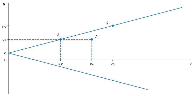
Figure 4: The figure shows the investment opportunity set available to an investor. The upper line determines the efficient frontier whereas the lower line is the set of inefficient portfolios. For a given portfolio A, there is a portfolio A' that has the same expected return as A but the lowest standard deviation. Both A' and Q are efficient portfolios.

Beta Pricing

• In Figure 4, portfolio A' is efficient, and therefore a combination of the tangency portfolio with the risk-free asset. r_{A'} = (1 - \beta) r_{f} + \beta r_{Q}.
• The residual \varepsilon = r_{A} - r_{A'} by construction has mean zero, implying that \operatorname{E}(r_{A}) = (1 - \beta) r_{f} + \beta \operatorname{E}(r_{Q}).
• The residual is also orthogonal to its projection r_{A'}, 0 = \operatorname{Cov}(\varepsilon, r_{A'}) = \operatorname{Cov}(r_{A} - r_{A'}, r_{A'}) = \beta \operatorname{Cov}(r_{A}, r_{Q}) - \beta^{2} \operatorname{V}(r_{Q}), or \beta = \frac{\operatorname{Cov}(r_{A}, r_{Q})}{\operatorname{V}(r_{Q})}.

Decomposing Returns

• Beta pricing implies that we can decompose returns into a systematic and a firm-specific part, r_{A} = (1 - \beta_{A}) r_{f} + \beta_{A} r_{Q} + \varepsilon_{A}.
• The residual \varepsilon_{A} is orthogonal to the tangency portfolio and therefore specific to the asset.
  • Firm-specific or idiosyncratic risk is diversifiable.
• The term \beta_{A} r_{Q} captures the systematic risk of the asset.
  • The higher the \beta, the more exposure the asset has to systematic risk.
  • Systematic risk is non-diversifiable.

Property 1 (Beta Pricing) Let Q be any mean-variance efficient portfolio. The return of any asset A can be decomposed into a systematic component and a firm-specific or idiosyncratic component, r_{A} = (1 - \beta_{A}) r_{f} + \beta_{A} r_{Q} + \varepsilon_{A}, \tag{1} where \beta_{A} = \frac{\operatorname{Cov}(r_{A}, r_{Q})}{\operatorname{V}(r_{Q})}. and \operatorname{E}(\varepsilon_{A}) = \operatorname{Cov}(\varepsilon_{A}, r_{Q}) = 0. Taking expectations, \operatorname{E}(r_{A}) = (1 - \beta_{A}) r_{f} + \beta_{A} \operatorname{E}(r_{Q}). \tag{2}

Pricing, Not Holdings

• Property 1 holds for any mean-variance efficient portfolio Q, whatever investors’ preferences and whatever the shape of the return distribution.
  • All it needs is that returns have finite means, variances, and covariances.
• The reason is diversification: the portfolio \beta_{A} r_{Q} + (1 - \beta_{A}) r_{f} matches A’s expected return while shedding \varepsilon_{A}.
  • The residual adds variance without adding expected return, so it earns no premium.
• Beta pricing says nothing about what investors should hold, only that the efficiency of Q prices every asset relative to it.
• The CAPM adds a single claim: that Q is the market portfolio M.