from getfactormodels import FamaFrenchFactors
import numpy as np
import pandas as pd
import matplotlib.pyplot as plt
import seaborn as sns
import statsmodels.formula.api as smf

sns.set_theme()Predicting Short-Rate Changes
This notebook studies the dynamics of the short-term interest rate using monthly data from 1926. We ask two questions: does the level of the risk-free rate predict its own future changes, and does the slope of the yield curve add predictive power beyond simple mean-reversion?
The first question is motivated by Vasicek (1977), one of the earliest equilibrium models of the term structure. The Vasicek model implies that the short rate follows a mean-reverting process, \[ \Delta r^f_{t + 1} = \alpha + \beta r^f_t + e_{t + 1}, \] where \(\Delta r^f_{t + 1} = r^f_{t + 1} - r^f_t\). Mean-reversion requires \(\beta < 0\): when the rate is above its long-run equilibrium \(r^* = -\alpha/\beta\), the expected change is negative, pulling it back down. We estimate this model on the full sample using Newey-West standard errors to correct for heteroskedasticity and autocorrelation.
Vasicek, Oldrich. 1977. “An Equilibrium Characterization of the Term Structure.” Journal of Financial Economics 5 (2): 177–88.
The second question is motivated by the expectations hypothesis of the term structure. If long rates are averages of expected future short rates, then the spread \(s_t = r^{10y}_t - r^f_t\) encodes the market’s expectation of where short rates are heading: a steep upward-sloping curve signals anticipated increases, an inverted curve signals anticipated cuts. We use month-end yields on the 3-month Treasury bill and the 10-year Treasury note from FRED (both available from 1962), augment the Vasicek regression with the lagged spread and the lagged change in the short rate, and then ask how the spread’s predictive power changes with the forecast horizon. Finally, we replace the spread with a forward rate and check whether any of these predictors would have helped someone forecasting in real time, using only the data available on each date.
Getting the Data
The short-term risk-free rate comes from the Fama-French data library via getfactormodels. The monthly RF series is reported as a decimal monthly return, so we multiply by 12 and by 100 to express it as an annualized percentage.
The dates need care. RF for month \(t\) is the return on a one-month Treasury bill bought at the end of month \(t-1\) and held through month \(t\). Its value is therefore known at the end of month \(t-1\): it is the interest rate set then, not a rate observed during month \(t\). Since we want \(r^f_t\) to be the rate known at date \(t\), we date each observation at the end of the previous month. Left with the Fama-French dates, the series would lag every other variable observed at month-end by one month, and a regression that mixes it with month-end yields would let a contemporaneous relation pass for a prediction.
start_date = '1926-01-01'

ff3 = (FamaFrenchFactors(model='3', frequency='m', start_date=start_date)
       .load()
       .to_pandas()
       )

rf = 12 * ff3[['RF']] * 100
# Date each rate at the end of the month in which it was set
rf.index = (pd.to_datetime(rf.index.astype(str))
            + pd.offsets.MonthEnd(0) - pd.offsets.MonthEnd(1))
For the term spread we need a short rate and a long rate observed on the same day. We download two daily series from FRED, the 3-month Treasury bill yield (DTB3) and the 10-year Treasury yield (DGS10), and keep the last observation of each month. FRED serves these series as CSV files that need no account or API key. FRED also publishes monthly averages of the same yields (TB3MS, GS10), but an average over the month is not known at month-end, so it would bring the timing problem back. We drop the current month, which is not over yet.
def fred_month_end(series):
    url = f'https://fred.stlouisfed.org/graph/fredgraph.csv?id={series}'
    daily = pd.read_csv(url, index_col=0, parse_dates=True,
                        na_values='.').iloc[:, 0]
    return daily.dropna().resample('ME').last()

last_month_end = pd.Timestamp.today().normalize() - pd.offsets.MonthEnd(1)

ts = (pd.concat({'RF': fred_month_end('DTB3'),
                 'T10': fred_month_end('DGS10')}, axis=1)
      .dropna()
      .loc[:last_month_end]
      )
ts['SPREAD'] = ts['T10'] - ts['RF']
ts['DELTA_RF'] = ts['RF'] - ts['RF'].shift(1)
First Look at the Data
We first plot the level of the 1-month Treasury rate from 1926.
plt.plot(rf.index, rf['RF'])
plt.title('1-Month Treasury Rate')
plt.ylabel('Rate (%)')
plt.show()
The previous plot shows that the risk-free rate is a persistent time-series, i.e. its level changes slowly through time. In econometrics we say that the level of the risk-free rate is highly autocorrelated. One way to see this is to plot \(r_{t+1}^f\) vs. \(r_{t}^f\).
sns.scatterplot(x=rf['RF'].shift(1), y=rf['RF'], alpha=0.5)
plt.title('Scatter Plot of $r_{t+1}^f$ vs. $r_{t}^f$')
plt.xlabel('$r_{t}^f$')
plt.ylabel('$r_{t+1}^f$')
plt.axhline(y=0, color='gray', linewidth=1)
plt.axvline(x=0, color='gray', linewidth=1)
plt.show()
This persistence creates a well-known problem called spurious regression. If two unrelated but persistent variables are regressed on each other, OLS will tend to find a highly significant relationship even though none exists in reality. The reason is mechanical: because each series moves slowly and stays close to its own past values, any two persistent series will appear correlated over a long sample simply by chance. Standard t-statistics are severely inflated, and R² can be misleadingly high. The solution is to work with the change in the variable rather than its level. First-differencing removes the slow drift that drives spurious correlation, leaving a stationary series that is amenable to standard regression inference.
rf['DELTA_RF'] = rf['RF'] - rf['RF'].shift(1)
sns.scatterplot(x=rf['RF'].shift(1), y=rf['DELTA_RF'], alpha=0.5)
plt.title('Scatter Plot of $\\Delta r_{t+1}^f$ vs. $r_{t}^f$')
plt.xlabel('$r_{t}^f$')
plt.ylabel('$\\Delta r_{t+1}^f$')
plt.axhline(y=0, color='gray', linewidth=1)
plt.axvline(x=0, color='gray', linewidth=1)
plt.show()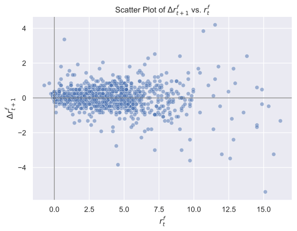
The scatter plot looks far less structured than the previous one. Whereas the level plot showed an almost perfect 45-degree line (a telltale sign of spurious persistence), the change plot is a diffuse cloud with no immediately obvious pattern. This is the right starting point for regression: any predictability we find in the changes will reflect genuine dynamics rather than the mechanical correlation induced by persistence.
We can verify this formally using the augmented Dickey-Fuller (ADF) test. The test asks whether the series has a unit root: a stochastic trend that makes the series wander without bound and never settle around a fixed mean. The null hypothesis is that a unit root is present (non-stationarity); the alternative is that the series is stationary (mean-reverting). A large negative ADF statistic and a small p-value lead us to reject the null and conclude stationarity. We expect to fail to reject for the level \(r^f_t\), consistent with the slow drift visible in the time-series plot, and to reject for the first difference \(\Delta r^f_t\), confirming that first-differencing is the right transformation before running regressions.
from statsmodels.tsa.stattools import adfuller

for label, series in [('RF level', rf['RF'].dropna()),
                      ('ΔRF change', rf['DELTA_RF'].dropna())]:
    adf = adfuller(series, autolag='AIC', result_object=True)
    print(f"{label}: ADF stat = {adf.statistic:.3f}, p-value = {adf.pvalue:.3f}")
RF level: ADF stat = -2.127, p-value = 0.234
ΔRF change: ADF stat = -8.208, p-value = 0.000A Simple Mean-Reversion Model
Although no pattern is visible to the naked eye, the Vasicek model predicts a subtle negative slope: when the rate is high, changes should be slightly negative on average, and vice versa. Detecting this requires regression. We estimate \[ \Delta r^f_{t + 1} = \alpha + \beta r^f_t + e_{t + 1}. \]
For this, we regress the change in the rates vs. the past level of the risk-free rate. We control for heteroscedasticity and autocorrelation of the residuals using the Newey-West correction (Newey and West 1987). Newey and West do not prescribe a number of lags; we use a common rule of thumb, the integer part of \(T^{1/4}.\)
Newey, Whitney K., and Kenneth D. West. 1987. “A Simple, Positive Semi-Definite, Heteroskedasticity and Autocorrelation Consistent Covariance Matrix.” Econometrica 55 (3): 703–8.
nw_lags = int(len(rf)**0.25)

results = (smf
           .ols('DELTA_RF ~ RF.shift(1)', data=rf)
           .fit(cov_type='HAC', cov_kwds={'maxlags': nw_lags})
           )

print(results.summary(slim=True))
OLS Regression Results
==============================================================================
Dep. Variable: DELTA_RF R-squared: 0.012
Model: OLS Adj. R-squared: 0.011
No. Observations: 1202 F-statistic: 7.089
Covariance Type: HAC Prob (F-statistic): 0.00786
===============================================================================
coef std err z P>|z| [0.025 0.975]
-------------------------------------------------------------------------------
Intercept 0.0784 0.023 3.409 0.001 0.033 0.123
RF.shift(1) -0.0239 0.009 -2.662 0.008 -0.041 -0.006
===============================================================================
Notes:
[1] Standard Errors are heteroscedasticity and autocorrelation robust (HAC) using 5 lags and without small sample correctionThe results show that both estimates for \(\alpha\) and \(\beta\) have p-values less than 1%, so we conclude that both \(\alpha\) and \(\beta\) are significant at the 1% level. The fact that \(\beta < 0\) implies that the risk-free rate is mean-reverting. To see this, note that the long-run equilibrium rate is \(r^* = -\alpha/\beta > 0\). When \(r^f_t > r^*\), the expected change \(\alpha + \beta r^f_t = \beta(r^f_t - r^*)\) is negative since \(\beta < 0\), pulling the rate back toward \(r^*\). The opposite holds when \(r^f_t < r^*\).
We can compute the implied equilibrium rate directly from the estimated coefficients:
alpha_hat = results.params['Intercept']
beta_hat  = results.params['RF.shift(1)']
r_star    = -alpha_hat / beta_hat
print(f"Implied long-run equilibrium: r* = {r_star:.2f}%")
print(f"Sample mean of RF:             {rf['RF'].mean():.2f}%")
Implied long-run equilibrium: r* = 3.28%
Sample mean of RF: 3.24%We can now add the line with the predicted values from the regression.
sns.regplot(x=rf['RF'].shift(1), y=rf['DELTA_RF'], scatter_kws={'alpha': 0.5})
plt.title('Scatter Plot of $\\Delta r_{t+1}^f$ vs. $r_{t}^f$')
plt.xlabel('$r_{t}^f$')
plt.ylabel('$\\Delta r_{t+1}^f$')
plt.axhline(y=0, color='gray', linewidth=1)
plt.axvline(x=0, color='gray', linewidth=1)
plt.show()
As expected, the slope coefficient of the line is negative.
Adding More Predictors
The simple model uses only the lagged level \(r^f_t\) to predict future rate changes. Two natural extensions suggest themselves. First, rate changes may be autocorrelated: if the Fed is in the middle of a tightening or easing cycle, last month’s move is likely to continue. Second, the slope of the yield curve (the difference between the 10-year yield and the short rate) encodes the market’s expectation of where short rates are heading. A steep curve signals anticipated rate increases; an inverted curve signals anticipated cuts. Both effects could improve predictive power beyond simple mean-reversion.
The term spread compares a long rate and a short rate, so both must be measured on the same day. In this section the short rate \(r^f_t\) is the month-end yield on the 3-month Treasury bill and the long rate \(r^{10y}_t\) is the month-end yield on the 10-year Treasury note, both from FRED. The 10-year series starts in January 1962, so the extended model uses a restricted sample. Before adding the new regressors, we re-estimate the simple model on this sample to see whether mean-reversion shows up there too.
We first plot the short rate, the 10-year yield, and the term spread over the restricted sample.
fig, axes = plt.subplots(2, 1, figsize=(10, 6), sharex=True)
axes[0].plot(ts.index, ts['RF'],  label='3-month T-bill yield')
axes[0].plot(ts.index, ts['T10'], label='10-year Treasury yield')
axes[0].set_ylabel('Rate (%)')
axes[0].legend()
axes[1].plot(ts.index, ts['SPREAD'], color='steelblue')
axes[1].axhline(0, color='gray', linewidth=1)
axes[1].set_ylabel('Spread (pp)')
plt.suptitle('Short Rate, 10-Year Yield, and Term Spread (1962 to present)')
plt.tight_layout()
plt.show()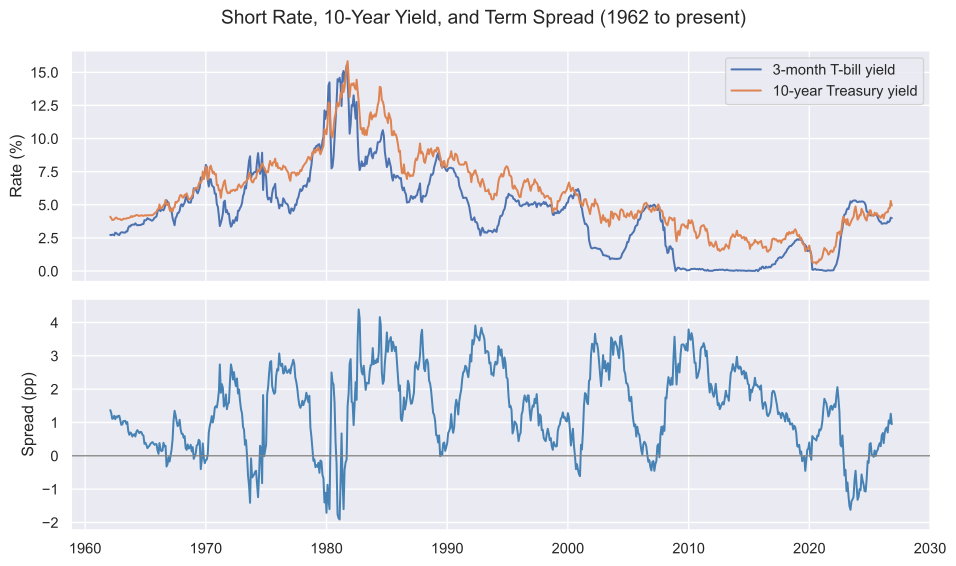
nw_lags_r = int(len(ts)**0.25)

results_r = (smf
             .ols('DELTA_RF ~ RF.shift(1)', data=ts)
             .fit(cov_type='HAC', cov_kwds={'maxlags': nw_lags_r})
             )

print(results_r.summary(slim=True))
OLS Regression Results
==============================================================================
Dep. Variable: DELTA_RF R-squared: 0.005
Model: OLS Adj. R-squared: 0.004
No. Observations: 777 F-statistic: 1.136
Covariance Type: HAC Prob (F-statistic): 0.287
===============================================================================
coef std err z P>|z| [0.025 0.975]
-------------------------------------------------------------------------------
Intercept 0.0457 0.032 1.410 0.158 -0.018 0.109
RF.shift(1) -0.0100 0.009 -1.066 0.287 -0.028 0.008
===============================================================================
Notes:
[1] Standard Errors are heteroscedasticity and autocorrelation robust (HAC) using 5 lags and without small sample correctionThe coefficient on RF.shift(1) keeps its negative sign on this sample, but it is smaller and not significant at conventional levels. Mean-reversion in the short rate is slow: with \(\hat\beta\) around \(-0.01\), the gap between the rate and its long-run level closes by about 1% a month, so it takes years to halve, while each month’s change is dominated by news about monetary policy. Detecting such slow reversion in one-month changes is hard even with 60 years of data.
We now extend the model to \[ \Delta r^f_{t+1} = \alpha + \beta r^f_t + \gamma \Delta r^f_t + \delta s_t + e_{t+1}. \]
The first new predictor is the lagged change \(\Delta r^f_t = r^f_t - r^f_{t-1}\), coded as DELTA_RF.shift(1). Applying .shift(1) to DELTA_RF lags it by one month, so that when predicting \(\Delta r^f_{t+1}\) we use \(\Delta r^f_t\), the change that just occurred. This tests whether rate changes are autocorrelated. For example, if the Fed begins a cutting cycle, rate decreases may persist over several months, making a positive \(\gamma\) plausible.
The second new predictor is the lagged term spread \(s_t = r^{10y}_t - r^f_t\) (SPREAD.shift(1)). The spread measures the slope of the yield curve: when long rates are well above short rates (\(s_t > 0\)), the market anticipates rising short rates, consistent with a positive \(\delta\). Using the spread rather than the 10-year yield directly avoids the high collinearity between RF.shift(1) and the level of the 10-year yield, since both series move closely together over the long run.
results2 = (smf
            .ols('DELTA_RF ~ RF.shift(1) + DELTA_RF.shift(1) + SPREAD.shift(1)', data=ts)
            .fit(cov_type='HAC', cov_kwds={'maxlags': nw_lags_r})
            )

print(results2.summary(slim=True))
OLS Regression Results
==============================================================================
Dep. Variable: DELTA_RF R-squared: 0.029
Model: OLS Adj. R-squared: 0.025
No. Observations: 776 F-statistic: 1.335
Covariance Type: HAC Prob (F-statistic): 0.262
=====================================================================================
coef std err z P>|z| [0.025 0.975]
-------------------------------------------------------------------------------------
Intercept 0.0148 0.043 0.344 0.731 -0.069 0.099
RF.shift(1) -0.0090 0.009 -1.008 0.314 -0.026 0.008
DELTA_RF.shift(1) 0.1549 0.101 1.528 0.126 -0.044 0.354
SPREAD.shift(1) 0.0189 0.016 1.147 0.251 -0.013 0.051
=====================================================================================
Notes:
[1] Standard Errors are heteroscedasticity and autocorrelation robust (HAC) using 5 lags and without small sample correctionNone of the three predictors is significant at the 5% level. The lagged change has the positive sign the policy-cycle argument suggests, and the spread has the positive sign the expectations hypothesis suggests, but both coefficients are within about one and a half standard errors of zero. Over the next month, the slope of the yield curve says little about where the short rate is going.
The following table compares all three specifications. Newey-West standard errors are reported in parentheses below each coefficient. The table uses standard significance codes: *** \(p < 0.01\), ** \(p < 0.05\), * \(p < 0.10\).
def fmt_coef(res, var):
    if var not in res.params:
        return ('', '')
    p = res.pvalues[var]
    stars = '***' if p < 0.01 else '**' if p < 0.05 else '*' if p < 0.10 else ''
    coef = f"{res.params[var]:.3f}{stars}"
    se   = f"({res.bse[var]:.3f})"
    return (coef, se)

specs = {
    'Simple (full, 1-month bill)':     results,
    'Simple (1962+, 3-month bill)':    results_r,
    'Extended (1962+, 3-month bill)':  results2,
}
coef_vars = ['Intercept', 'RF.shift(1)', 'DELTA_RF.shift(1)', 'SPREAD.shift(1)']

# Build multi-row index: coefficient row then SE row for each variable
index_labels = []
for v in coef_vars:
    index_labels += [v, '']

table = {}
for name, res in specs.items():
    col = []
    for v in coef_vars:
        coef, se = fmt_coef(res, v)
        col += [coef, se]
    table[name] = col

df_table = pd.DataFrame(table, index=index_labels)
df_table.loc['N']  = {name: str(int(res.nobs))        for name, res in specs.items()}
df_table.loc['R²'] = {name: f"{res.rsquared:.3f}"     for name, res in specs.items()}

display(df_table)| Simple (full, 1-month bill) | Simple (1962+, 3-month bill) | Extended (1962+, 3-month bill) | |
|---|---|---|---|
| Intercept | 0.078*** | 0.046 | 0.015 |
| (0.023) | (0.032) | (0.043) | |
| RF.shift(1) | -0.024*** | -0.010 | -0.009 |
| (0.009) | (0.009) | (0.009) | |
| DELTA_RF.shift(1) | 0.155 | ||
| (0.101) | |||
| SPREAD.shift(1) | 0.019 | ||
| (0.016) | |||
| N | 1202 | 777 | 776 |
| R² | 0.012 | 0.005 | 0.029 |
The table highlights two findings. First, the evidence for mean-reversion in one-month changes depends on the sample: it is significant over the full sample of one-month bill rates since 1926, but not over the 3-month bill yields since 1962. Second, adding the lagged change and the spread raises R² on the restricted sample only to about 3%. At a one-month horizon, changes in the short rate are close to unpredictable.
Longer Horizons
The expectations hypothesis is a statement about the whole path of short rates until the long bond matures, not about next month. A 10-year yield above the bill rate says that short rates are expected to be higher on average over the coming years; it says little about which month the increases arrive. We therefore regress the change in the short rate over the next \(k\) months on today’s spread, \[ r^f_{t+k} - r^f_t = a_k + b_k s_t + e_{t+k}, \] for horizons from one month to three years. With monthly data and \(k > 1\), consecutive observations share \(k - 1\) months of the same rate changes, so the residuals are autocorrelated by construction. The Newey-West correction is designed for this kind of autocorrelation, and its number of lags should cover the overlap; we use the larger of \(k\) and \(T^{1/4}\).
rows = []
for k in [1, 3, 6, 12, 24, 36]:
    d = pd.DataFrame({'CHANGE': ts['RF'].shift(-k) - ts['RF'],
                      'SPREAD': ts['SPREAD']}).dropna()
    lags = max(k, int(len(d)**0.25))
    res = (smf
           .ols('CHANGE ~ SPREAD', data=d)
           .fit(cov_type='HAC', cov_kwds={'maxlags': lags})
           )
    rows.append({'Horizon (months)': k,
                 'Slope': f"{res.params['SPREAD']:.3f}",
                 't-stat': f"{res.tvalues['SPREAD']:.2f}",
                 'R²': f"{res.rsquared:.3f}",
                 'N': int(res.nobs)})

display(pd.DataFrame(rows).set_index('Horizon (months)'))| Slope | t-stat | R² | N | |
|---|---|---|---|---|
| Horizon (months) | ||||
| 1 | 0.017 | 1.06 | 0.002 | 777 |
| 3 | 0.059 | 1.37 | 0.008 | 775 |
| 6 | 0.121 | 1.83 | 0.017 | 772 |
| 12 | 0.230 | 2.00 | 0.030 | 766 |
| 24 | 0.591 | 2.67 | 0.089 | 754 |
| 36 | 0.829 | 2.98 | 0.125 | 742 |
The slope rises with the horizon. At one and three months the spread has no reliable predictive power. From about a year onward the coefficient is positive and roughly two to three standard errors from zero, and R² climbs to around 10% at two to three years. A steep yield curve does forecast rising short rates, but over years, not months. The overlap also means there are far fewer independent observations than \(N\) suggests (the sample since 1962 holds only about 21 non-overlapping three-year periods), so the long-horizon t-statistics deserve some caution.
Forward Rates
The 10-year spread is a blunt tool for forecasting the bill rate one year ahead. The 10-year yield reflects expected short rates over the next ten years, plus a term premium, while we only care about the next twelve months. A sharper measure is the forward rate: the interest rate an investor can lock in today, by buying one Treasury bond and selling another of a different maturity, for a loan that starts one year from now. If forward rates are expected future short rates, as the expectations hypothesis says, the forward spread \(f_t - r^f_t\) is the market’s forecast of how much the short rate will change over the next year.
Forward rates are not quoted directly; they have to be computed from the whole yield curve. The Federal Reserve publishes such a curve, estimated by Gürkaynak et al. (2007), every day since 1961, as a CSV file. The column SVENF01 is the forward rate for a very short loan starting in exactly one year. It is continuously compounded, while the bill yield is not; the gap between the two conventions is small and nearly constant, so the regression intercept absorbs it. The Fed’s server rejects requests that do not identify a browser, so we pass a User-Agent header. The file is about 17 MB, so the download takes a few seconds.
Gürkaynak, Refet S., Brian Sack, and Jonathan H. Wright. 2007. “The U.S. Treasury Yield Curve: 1961 to the Present.” Journal of Monetary Economics 54: 2291–304.
gsw_url = 'https://www.federalreserve.gov/data/yield-curve-tables/feds200628.csv'
gsw = pd.read_csv(gsw_url, skiprows=9, index_col=0, parse_dates=True,
                  usecols=['Date', 'SVENF01'],
                  storage_options={'User-Agent': 'Mozilla/5.0'})

ts['FWD'] = gsw['SVENF01'].dropna().resample('ME').last()
ts['FWD_SPREAD'] = ts['FWD'] - ts['RF']
The two spreads move together, but not one-for-one: the forward spread reacts to the near end of the curve, the 10-year spread to the whole curve.
plt.plot(ts.index, ts['SPREAD'], label='10-year yield minus bill')
plt.plot(ts.index, ts['FWD_SPREAD'], label='1-year forward rate minus bill')
plt.axhline(0, color='gray', linewidth=1)
plt.ylabel('Spread (pp)')
plt.title('Two Measures of the Slope of the Yield Curve')
plt.legend()
plt.show()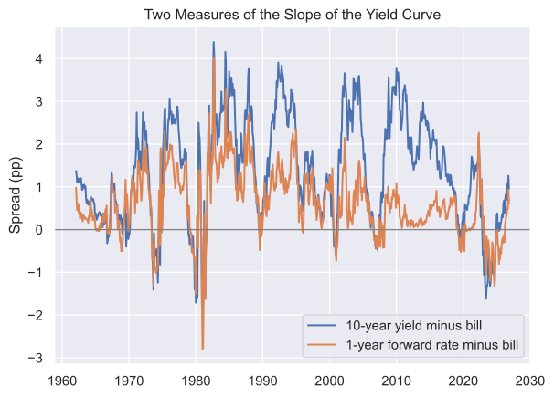
We now compare three predictors of the change in the bill rate over the next 12 months: the level of the rate itself (mean-reversion), the 10-year spread, and the forward spread. Each regression has a single predictor, so we can compare their fit directly.
k = 12
rows = []
for predictor in ['RF', 'SPREAD', 'FWD_SPREAD']:
    d = pd.DataFrame({'CHANGE': ts['RF'].shift(-k) - ts['RF'],
                      'X': ts[predictor]}).dropna()
    res = (smf
           .ols('CHANGE ~ X', data=d)
           .fit(cov_type='HAC', cov_kwds={'maxlags': k})
           )
    rows.append({'Predictor': predictor,
                 'Slope': f"{res.params['X']:.3f}",
                 't-stat': f"{res.tvalues['X']:.2f}",
                 'R²': f"{res.rsquared:.3f}",
                 'N': int(res.nobs)})

display(pd.DataFrame(rows).set_index('Predictor'))| Slope | t-stat | R² | N | |
|---|---|---|---|---|
| Predictor | ||||
| RF | -0.143 | -2.19 | 0.072 | 766 |
| SPREAD | 0.230 | 2.00 | 0.030 | 766 |
| FWD_SPREAD | 0.389 | 1.93 | 0.034 | 766 |
All three slopes have the expected sign and are about two standard errors from zero. The level of the rate has the highest R², and the two spreads are close to each other. Judged by this table alone, mean-reversion looks like the best predictor.
Forecasting Out of Sample
The R² in the table measures how well each regression fits the data used to estimate it. That is not what a forecaster faces. Someone forecasting the bill rate in 1990 could estimate the regression only with data up to 1990, and the slope estimated with data through 2026 was not available to them. A predictor can fit the past well and still forecast badly, because the regression adapts to the sample it was estimated on.
To mimic a real forecaster, we step through the sample one month at a time. On each date we estimate the regression using only the 12-month changes already observed by then, and forecast the next 12-month change with today’s value of the predictor. We compare these forecasts with a simple benchmark: the average 12-month change observed so far. The out-of-sample R², \[ R^2_{\text{OOS}} = 1 - \frac{\sum_t (\text{actual}_t - \text{regression forecast}_t)^2}{\sum_t (\text{actual}_t - \text{historical mean}_t)^2}, \] is positive when the regression forecasts better than the historical mean and negative when it forecasts worse. Unlike the usual R², it can be negative. Welch and Goyal (2008) use this comparison for stock returns and find that most variables proposed in the literature to predict the equity premium forecast worse than the historical mean out of sample, and their performance is unstable over time.
Welch, Ivo, and Amit Goyal. 2008. “A Comprehensive Look at the Empirical Performance of Equity Premium Prediction.” Review of Financial Studies 21 (4): 1455–508.
One detail matters for the timing. The 12-month change that starts in month \(s\) is only known in month \(s + 12\). So on date \(t\) we can only use the changes that started 12 months before \(t\) or earlier; using later ones would let the forecaster peek at the future.
def oos_r2(data, predictor, k, start):
    d = pd.DataFrame({'y': data['RF'].shift(-k) - data['RF'],
                      'x': data[predictor]}).dropna()
    errors_model, errors_mean = [], []
    for date in d.loc[start:].index:
        # Only changes already observed on this date can be used
        past = d.loc[:date - pd.offsets.MonthEnd(k)]
        slope, intercept = np.polyfit(past['x'], past['y'], 1)
        errors_model.append(d.at[date, 'y'] - (intercept + slope * d.at[date, 'x']))
        errors_mean.append(d.at[date, 'y'] - past['y'].mean())
    return 1 - np.sum(np.square(errors_model)) / np.sum(np.square(errors_mean))

rows = []
for predictor in ['RF', 'SPREAD', 'FWD_SPREAD']:
    rows.append({'Predictor': predictor,
                 'Forecasts from 1975': f"{oos_r2(ts, predictor, k, '1975'):.3f}",
                 'Forecasts from 1985': f"{oos_r2(ts, predictor, k, '1985'):.3f}"})

display(pd.DataFrame(rows).set_index('Predictor'))| Forecasts from 1975 | Forecasts from 1985 | |
|---|---|---|
| Predictor | ||
| RF | -0.115 | -0.064 |
| SPREAD | -0.056 | 0.012 |
| FWD_SPREAD | -0.019 | 0.050 |
The ranking flips. The level of the rate, which had the best in-sample fit, forecasts worse than the historical mean whichever date the forecasts start. The forward spread is the best of the three, but it beats the historical mean only when the forecasts start in 1985. Starting in 1975, no predictor beats the simple average.
To see why the starting date matters, we estimate the two spread regressions separately before and after 1985.
rows = []
for label, sub in [('1962-1984', ts.loc['1962':'1984']),
                   ('1985-present', ts.loc['1985':])]:
    for predictor in ['SPREAD', 'FWD_SPREAD']:
        d = pd.DataFrame({'CHANGE': sub['RF'].shift(-k) - sub['RF'],
                          'X': sub[predictor]}).dropna()
        res = (smf
               .ols('CHANGE ~ X', data=d)
               .fit(cov_type='HAC', cov_kwds={'maxlags': k})
               )
        rows.append({'Period': label, 'Predictor': predictor,
                     'Slope': f"{res.params['X']:.3f}",
                     't-stat': f"{res.tvalues['X']:.2f}",
                     'R²': f"{res.rsquared:.3f}"})

display(pd.DataFrame(rows).set_index(['Period', 'Predictor']))| Slope | t-stat | R² | ||
|---|---|---|---|---|
| Period | Predictor | |||
| 1962-1984 | SPREAD | 0.374 | 1.74 | 0.047 |
| FWD_SPREAD | 0.321 | 1.12 | 0.021 | |
| 1985-present | SPREAD | 0.296 | 2.27 | 0.069 |
| FWD_SPREAD | 0.664 | 2.80 | 0.108 |
Before 1985 neither spread predicts the bill rate reliably. That period includes the years 1979 to 1982, when the Fed targeted the growth of the money supply and let the short rate swing by several percentage points within a few months, moves the yield curve did not anticipate. Since 1985 the forward spread predicts much better, and better than the 10-year spread. A forecaster starting in 1975 spends the first decade with a regression estimated on the old relation, and those forecasts are poor enough to undo the later gains.
Three lessons carry over to any forecasting exercise. A t-statistic around two in sample does not make a useful forecast. Out-of-sample tests, which use only the data available on each date, are the honest check. And relations in economic data change over time, so a conclusion that depends on where the sample starts or ends deserves less weight than one that does not.
Campbell and Shiller (1991) examine almost every pair of maturities between one month and ten years and find what they call an apparent paradox. A steep yield curve forecasts rising short rates over the long term, the direction the expectations hypothesis predicts, and when the long bond matures in more than three or four years the slope coefficient is close to the value of one that the hypothesis implies; for shorter maturities it falls well below one. Over short horizons, however, the spread forecasts the yield on the long bond in the wrong direction: a steep curve predicts falling, not rising, long yields. They describe the pattern as a spread that points in the direction the expectations hypothesis implies but is larger than expected changes in short rates justify, and offer two explanations: risk premia that vary over time together with expected changes in short rates, or long rates that react too sluggishly to sudden moves in the short rate. Fama and Bliss (1987) find a similar horizon pattern with forward rates: one-year forward rates on 1- to 5-year Treasury bonds have little power to forecast the one-year rate a year ahead, but forecast its changes two to four years ahead, and forecast power increases with the horizon. They attribute this to a slow mean-reverting tendency in interest rates, and they find that expected term premiums vary through time. Mishkin (1988) uses forward rates on Treasury bills, with standard errors corrected for overlapping observations, and finds that the term structure predicts changes in the one-month rate several months ahead. Its predictive power was generally higher after the Fed changed its operating procedures in October 1979 and again in October 1982, an early sign of the instability in the subsample table above. Taken together, the literature supports the positive coefficients on the spread found here at horizons of a year or more.
Campbell, John Y., and Robert J. Shiller. 1991. “Yield Spreads and Interest Rate Movements: A Bird’s Eye View.” Review of Economic Studies 58 (3): 495–514.
Fama, Eugene F., and Robert R. Bliss. 1987. “The Information in Long-Maturity Forward Rates.” American Economic Review 77 (4): 680–92.
Mishkin, Frederic S. 1988. “The Information in the Term Structure: Some Further Results.” Journal of Applied Econometrics 3 (4): 307–14.
Practice Problems
Problem 1 What does it mean that interest rates are persistent?
Solution
Persistence relates to the fact that the time-series changes slowly over time. A scatter plot of a persistent variable \(x_{t}\) vs. \(x_{t-1}\) will look as if there is predictability, although this is just spurious.Problem 2 Using the estimated \(\hat\alpha\) and \(\hat\beta\) from the simple mean-reversion model on the full sample, compute the implied long-run equilibrium rate \(r^* = -\hat\alpha/\hat\beta\). How does \(r^*\) compare to the sample mean of the short rate? What does any discrepancy tell you about the finite-sample behavior of the model?