import pandas as pd
from getfactormodels import FamaFrenchFactors, CarhartFactors
import yfinance as yf
import statsmodels.formula.api as smf
import matplotlib.pyplot as plt
import seaborn as sns

sns.set_theme()Analyzing Mutual Fund Returns
Mutual Funds
One of the main uses of asset pricing models is to analyze the performance of mutual funds. A mutual fund is a type of investment vehicle that pools money from many individual investors to purchase a diversified portfolio of stocks, bonds, or other securities. The fund is managed by a professional portfolio manager who invests the money in accordance with the fund’s investment objectives and strategy.
There are many different types of mutual funds, including equity funds, bond funds, balanced funds, index funds, and specialty funds. Each type of fund has its own investment strategy and risk profile, and investors should carefully consider their investment objectives and risk tolerance before choosing a mutual fund to invest in.
In this notebook we will analyze the Fidelity Value Fund (Ticker: FDVLX). According to the fund description, the fund invests in securities of companies that possess valuable fixed assets or that the fund manager believes are undervalued in the marketplace in relation to factors such as assets, earnings, or growth potential (stocks of these companies are often called “value” stocks). Normally investing primarily in common stocks.
We are interested in two related questions. First, how are the fund’s returns generated? That is, does the fund tilt toward small or large stocks, value or growth stocks, profitable firms, conservative or aggressive investors, and past winners or losers? Second, after accounting for these systematic exposures, does the fund earn a positive alpha, evidence of genuine skill beyond passive factor exposure?
One important caveat before we begin: we are studying a fund that still exists and has a long return history available. This introduces survivorship bias: funds that performed poorly were more likely to be closed or merged, and are absent from our sample. Focusing on surviving funds therefore tends to overstate the average alpha in the mutual fund industry. The Fama-French factors, by contrast, are constructed from a CRSP universe that includes delisted firms, so the factor data does not share this problem. Keep this asymmetry in mind when interpreting the alpha estimate: selecting a fund because it survived tilts the evidence toward good performance, so a negative alpha for a surviving fund is all the more telling.
The Augmented Five-Factor Model
We will estimate the Fama-French five-factor model augmented by the momentum factor, \[ R_{i} = a_{i} + b_{i} R_{m} + s_{i} \mathit{SMB} + h_{i} \mathit{HML} + r_{i} \mathit{RMW} + c_{i} \mathit{CMA} + m_{i} \mathit{MOM} + e_{i} \] where \(R_{i} = r_{i} - r_{f}\) represents the monthly excess returns for security \(i\) over the risk-free rate, and \(R_{m} = r_{m} - r_{f}\) represents the monthly excess returns of the market.
The estimation of \(a_{i}\), which is commonly called the alpha, now controls for many important sources of variation in the investment opportunity set. If the model is correct then the alpha should be close to zero.
The different loadings on the factors also have a clear interpretation. For a mutual fund we have that: - \(b_{i} < 1\) implies that the fund has less systematic risk than the market whereas a \(b_{i} > 1\) implies that the fund takes more systematic risk than the market. - \(s_{i} > 0\) implies that the fund loads mostly on small stocks whereas \(s_{i} < 0\) implies that the fund loads on large stocks. - \(h_{i} > 0\) implies that the fund loads on value stocks whereas \(h_{i} < 0\) implies that the fund loads on growth stocks. - \(r_{i} > 0\) implies that the fund loads on stocks with robust operating profitability whereas \(r_{i} < 0\) implies that the fund loads on stocks with weak operating profitability. - \(c_{i} > 0\) implies that the fund loads on stocks with low investment whereas \(c_{i} < 0\) implies that the fund loads on stocks with high investments. - \(m_{i} > 0\) implies that the fund loads on winners whereas \(m_{i} < 0\) implies that the fund loads on losers, i.e. follows a contrarian strategy.
The CAPM can be obtained by restricting \(s_{i} = 0\), \(h_{i} = 0\), \(r_{i} = 0\), \(c_{i} = 0\), and \(m_{i} = 0\). Other nested models can be obtained in a similar way.
Python Packages
Before starting, do not forget to reinstall getfactormodels if you are using a new session in Google Colab:
!pip install getfactormodels --quietGetting the Factors
We will download data starting December 1995 until January 2026.
start_date = "1995-12-01"
end_date = "2026-01-01"
ticker = "FDVLX"
The following code summarizes what we did in the previous notebook. Note that getfactormodels already returns factors in decimal form, so they are directly comparable to the fund returns computed by pct_change().
ff = (
    FamaFrenchFactors(model='5', frequency='m', start_date=start_date, end_date=end_date)
    .load()
    .to_pandas()
    .rename(columns={"Mkt-RF": "RMRF"})
)

mom = (
    CarhartFactors(frequency='m', start_date=start_date, end_date=end_date)
    .load()
    .to_pandas()
    [["MOM"]]
)

ff_mom = pd.merge(left=ff, right=mom, left_index=True, right_index=True)
ff_mom.index = pd.to_datetime(ff_mom.index).to_period('M')
display(ff_mom)| RMRF | SMB | HML | RMW | CMA | RF | MOM | |
|---|---|---|---|---|---|---|---|
| date | |||||||
| 1995-12 | 0.0104 | 0.0065 | 0.0024 | -0.0144 | 0.0302 | 0.0049 | 0.0250 |
| 1996-01 | 0.0226 | -0.0264 | 0.0045 | 0.0028 | 0.0229 | 0.0043 | 0.0055 |
| 1996-02 | 0.0133 | 0.0177 | -0.0105 | 0.0017 | -0.0188 | 0.0039 | 0.0057 |
| 1996-03 | 0.0074 | 0.0157 | 0.0042 | 0.0147 | -0.0095 | 0.0039 | -0.0185 |
| 1996-04 | 0.0205 | 0.0470 | -0.0396 | -0.0020 | -0.0202 | 0.0046 | -0.0096 |
| ... | ... | ... | ... | ... | ... | ... | ... |
| 2025-08 | 0.0184 | 0.0482 | 0.0437 | -0.0069 | 0.0197 | 0.0038 | -0.0361 |
| 2025-09 | 0.0339 | -0.0217 | -0.0105 | -0.0201 | -0.0227 | 0.0033 | 0.0462 |
| 2025-10 | 0.0196 | -0.0135 | -0.0318 | -0.0525 | -0.0407 | 0.0037 | 0.0016 |
| 2025-11 | -0.0013 | 0.0148 | 0.0376 | 0.0143 | 0.0064 | 0.0030 | -0.0172 |
| 2025-12 | -0.0036 | -0.0020 | 0.0240 | 0.0032 | 0.0040 | 0.0034 | -0.0240 |
361 rows × 7 columns
Getting the Data Ready
Fund Returns
We download the adjusted close price series from Yahoo! Finance. Even though returns are computed internally within the fund by reinvesting dividends from its holdings, the fund itself makes periodic distributions (dividends and capital gains) to shareholders that cause the NAV to drop on the ex-distribution date. Using adjusted close prices ensures these distributions are captured in the return computation. Note that all subsequent conclusions rely on this adjustment being accurate: if any distributions are missing or incorrectly recorded, the alpha estimate could be either overstated or understated. For the two funds in this notebook, the monthly returns computed this way match those in the CRSP mutual fund database, the standard academic source, to within 0.5% in every month.
stock = yf.download(tickers=ticker, start=start_date, end=end_date, auto_adjust=True, progress=False, multi_level_index=False).loc[:, ["Close"]]
ax = stock.plot(title="Price of " + ticker)
plt.show()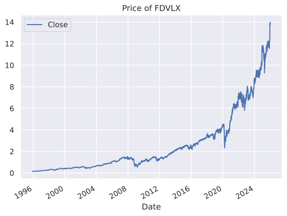
We compute monthly returns and use RET to denote the column containing the returns.
ret = stock.resample("ME").last().pct_change()
ret.index = ret.index.to_period("M")
ret = ret.rename(columns={"Close": "RET"})
ax = ret.plot(title="Monthly Return on " + ticker)
plt.show()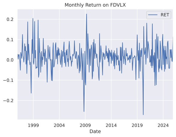
Merge with the Factors
Finally, we merge the returns series that we want to analyze with the six factors. Additionally, we compute excess returns for the security.
merged = (
    pd.merge(left=ret, right=ff_mom, left_index=True, right_index=True)
    .assign(RETRF=lambda d: d["RET"] - d["RF"])
    .drop(columns=["RET", "RF"])
    .dropna()
)
display(merged)| RMRF | SMB | HML | RMW | CMA | MOM | RETRF | |
|---|---|---|---|---|---|---|---|
| Date | |||||||
| 1996-01 | 0.0226 | -0.0264 | 0.0045 | 0.0028 | 0.0229 | 0.0055 | 0.022694 |
| 1996-02 | 0.0133 | 0.0177 | -0.0105 | 0.0017 | -0.0188 | 0.0057 | -0.000565 |
| 1996-03 | 0.0074 | 0.0157 | 0.0042 | 0.0147 | -0.0095 | -0.0185 | 0.021124 |
| 1996-04 | 0.0205 | 0.0470 | -0.0396 | -0.0020 | -0.0202 | -0.0096 | 0.021721 |
| 1996-05 | 0.0236 | 0.0324 | -0.0091 | 0.0006 | -0.0034 | 0.0160 | 0.009366 |
| ... | ... | ... | ... | ... | ... | ... | ... |
| 2025-08 | 0.0184 | 0.0482 | 0.0437 | -0.0069 | 0.0197 | -0.0361 | 0.046998 |
| 2025-09 | 0.0339 | -0.0217 | -0.0105 | -0.0201 | -0.0227 | 0.0462 | -0.006753 |
| 2025-10 | 0.0196 | -0.0135 | -0.0318 | -0.0525 | -0.0407 | 0.0016 | -0.012016 |
| 2025-11 | -0.0013 | 0.0148 | 0.0376 | 0.0143 | 0.0064 | -0.0172 | 0.035435 |
| 2025-12 | -0.0036 | -0.0020 | 0.0240 | 0.0032 | 0.0040 | -0.0240 | 0.015366 |
360 rows × 7 columns
Estimating the Model
CAPM
We start by estimating a CAPM regression, \[ R_{i} = a_{i} + b_{i} R_{m} + e_{i} \]
results = smf.ols("RETRF ~ RMRF", data=merged).fit()
print(results.summary(slim=True))
OLS Regression Results
==============================================================================
Dep. Variable: RETRF R-squared: 0.731
Model: OLS Adj. R-squared: 0.730
No. Observations: 360 F-statistic: 973.8
Covariance Type: nonrobust Prob (F-statistic): 3.64e-104
==============================================================================
coef std err t P>|t| [0.025 0.975]
------------------------------------------------------------------------------
Intercept -0.0003 0.002 -0.217 0.828 -0.003 0.003
RMRF 1.0555 0.034 31.206 0.000 0.989 1.122
==============================================================================
Notes:
[1] Standard Errors assume that the covariance matrix of the errors is correctly specified.The CAPM alpha is slightly negative (a = -0.0003 per month) and far from statistically significant (p-value = 0.83). Measured against the market alone, the fund earned about what its market beta of 1.06 would predict.
The Augmented Five-Factor Model
results = smf.ols("RETRF ~ RMRF + SMB + HML + RMW + CMA + MOM", data=merged).fit()
print(results.summary(slim=True))
OLS Regression Results
==============================================================================
Dep. Variable: RETRF R-squared: 0.909
Model: OLS Adj. R-squared: 0.908
No. Observations: 360 F-statistic: 590.8
Covariance Type: nonrobust Prob (F-statistic): 1.04e-180
==============================================================================
coef std err t P>|t| [0.025 0.975]
------------------------------------------------------------------------------
Intercept -0.0020 0.001 -2.128 0.034 -0.004 -0.000
RMRF 1.0639 0.023 45.934 0.000 1.018 1.110
SMB 0.3544 0.033 10.737 0.000 0.290 0.419
HML 0.3821 0.039 9.822 0.000 0.306 0.459
RMW 0.3570 0.042 8.542 0.000 0.275 0.439
CMA 0.1018 0.055 1.837 0.067 -0.007 0.211
MOM -0.1600 0.020 -7.984 0.000 -0.199 -0.121
==============================================================================
Notes:
[1] Standard Errors assume that the covariance matrix of the errors is correctly specified.After controlling for the other factors, the alpha falls to -0.0020 per month (p-value = 0.034): it is negative and statistically significant at the 5% level.
We learn the following from the coefficient estimates.
| Factor | Coefficient | Significance | Interpretation |
|---|---|---|---|
| SMB | 0.3544 | 1% | The fund invested in small stocks |
| HML | 0.3821 | 1% | The fund invested in value stocks |
| RMW | 0.3570 | 1% | The fund invested in stocks with strong profitability |
| CMA | 0.1018 | 10% | The fund tilted mildly toward low-investment (conservative) firms |
| MOM | -0.1600 | 1% | The fund followed a contrarian strategy, tilting toward past losers |
Therefore, the results from the regression agree with the fund description. The fund loads positively and significantly on HML, consistent with a value strategy. The positive SMB loading suggests the fund tilts toward smaller stocks within the value universe. The negative momentum loading is typical for value strategies, since value stocks tend to be recent underperformers.
The alpha tells a less flattering story. Against the market alone the fund looked average, but its returns came from exposures to small, value, and profitable stocks that a combination of the factor portfolios would have earned too. Once we account for those exposures, the fund underperforms by about 0.20% per month (\(0.20 \times 12 \approx 2.4\%\) per year), and the estimate is statistically significant at the 5% level. Part of the gap is cost: fund returns are measured after fees and trading expenses, which the factor portfolios do not pay. The fund delivers on its mandate, a value tilt, but the evidence gives no sign of skill beyond that tilt.
Practice Problems
Problem 1 In this problem we will analyze the Federated Hermes MDT Mid Cap Growth Fund Institutional Shares (Ticker: FGSIX) using data from the launch of this share class in January 2010 until January 2026.
- Download the Fama-French and momentum factors for the period.
- Download the fund net asset values (NAV) and compute monthly fund returns.
- Merge both datasets in a single dataframe.
- Run a regression of monthly fund returns on the Fama-French and momentum factors.
- Has the fund outperformed or underperformed the augmented Fama-French factor model during the period?
- Do the factor loadings on value and size correspond to the fund description?
- Does the fund load a lot on momentum?
Solution
The following assumes that you already have loaded the relevant libraries. We start by defining the start and end dates, and the ticker of the fund.
start_date = "2010-01-01"
end_date = "2026-01-01"
ticker = "FGSIX"
We can now proceed to get the Fama-French factors.
ff = (
    FamaFrenchFactors(model='5', frequency='m', start_date=start_date, end_date=end_date)
    .load()
    .to_pandas()
    .rename(columns={"Mkt-RF": "RMRF"})
)

mom = (
    CarhartFactors(frequency='m', start_date=start_date, end_date=end_date)
    .load()
    .to_pandas()
    [["MOM"]]
)

ff_mom = pd.merge(left=ff, right=mom, left_index=True, right_index=True)
ff_mom.index = pd.to_datetime(ff_mom.index).to_period('M')
We can now get the data for the fund and merge it with the Fama-French factors.
stock = yf.download(tickers=ticker, start=start_date, end=end_date, auto_adjust=True, progress=False, multi_level_index=False).loc[:, ["Close"]]
ret = stock.resample("ME").last().pct_change()
ret.index = ret.index.to_period("M")
ret = ret.rename(columns={"Close": "RET"})
merged = ( pd.merge(left=ret, right=ff_mom, left_index=True, right_index=True) .assign(RETRF=lambda d: d["RET"] - d["RF"]) .drop(columns=["RET", "RF"]) .dropna() )We can now run the regression of fund returns on the six factors.
results = smf.ols("RETRF ~ RMRF + SMB + HML + RMW + CMA + MOM", data=merged).fit()
print(results.summary(slim=True))
OLS Regression Results ============================================================================== Dep. Variable: RETRF R-squared: 0.892 Model: OLS Adj. R-squared: 0.889 No. Observations: 191 F-statistic: 254.1 Covariance Type: nonrobust Prob (F-statistic): 3.23e-86 ============================================================================== coef std err t P>|t| [0.025 0.975] ------------------------------------------------------------------------------ Intercept -0.0010 0.001 -0.772 0.441 -0.004 0.002 RMRF 1.0961 0.033 33.517 0.000 1.032 1.161 SMB 0.2755 0.058 4.710 0.000 0.160 0.391 HML -0.1260 0.056 -2.240 0.026 -0.237 -0.015 RMW 0.0107 0.071 0.149 0.881 -0.130 0.151 CMA -0.1570 0.082 -1.904 0.059 -0.320 0.006 MOM 0.1079 0.041 2.609 0.010 0.026 0.190 ============================================================================== Notes: [1] Standard Errors assume that the covariance matrix of the errors is correctly specified.The alpha of the fund is negative (-0.10% per month) but far from statistically significant (p-value = 0.44). The fund has neither outperformed nor underperformed the augmented Fama-French model in a statistically reliable way.
The SMB coefficient is positive (0.2755) and the HML coefficient negative (-0.1260), both significant at the 5% level: the fund tilts toward smaller stocks and toward growth stocks. Both signs are consistent with the fund’s description as a mid-cap growth fund.
The momentum loading is positive (0.1079) and significant at the 1% level (p = 0.010), but small: a 1% return on the momentum factor moves the fund’s return by only about 0.1%. The fund tilts modestly toward past winners.