The Momentum Factor

Modified

November 9, 2026

Theoretical Background

While Fama and French (1993) established that size and value captured important dimensions of expected returns, subsequent research showed that additional patterns in the cross-section of returns remained unexplained. The most prominent is momentum: Fama and French (1996) find that their three-factor model captures most of the anomalies they examine, except for the continuation of short-term returns.

Fama, Eugene F., and Kenneth R. French. 1993. “Common Risk Factors in the Returns on Stocks and Bonds.” Journal of Financial Economics 33 (1): 3–56.

Fama, Eugene F., and Kenneth R. French. 1996. “Multifactor Explanations of Asset Pricing Anomalies.” Journal of Finance 51 (1): 55–84.

Jegadeesh and Titman (1993) document that a portfolio that buys past winners and sells past losers earns significant positive returns over 3- to 12-month holding periods, and that these returns are not explained by the strategy’s systematic (market) risk or by delayed stock price reactions to common factors. Momentum refers to the tendency of stocks that have performed well (or poorly) in the recent past to continue to perform well (or poorly) in the future.

Carhart (1997) expanded on the momentum phenomenon documented by Jegadeesh and Titman (1993) by incorporating it into a four-factor asset pricing model. In addition to the market risk factor, Carhart (1997) added three additional factors: size (SMB), book-to-market (HML), and momentum (MOM).

Jegadeesh, Narasimhan, and Sheridan Titman. 1993. “Returns to Buying Winners and Selling Losers: Implications for Stock Market Efficiency.” Journal of Finance 48 (1): 65–91.

The momentum factor is constructed by using six value-weighted portfolios formed on size and prior (2-12) returns. The portfolios, which are formed monthly, are the intersections of 2 portfolios formed on size (market equity, ME) and 3 portfolios formed on prior (2-12) return. The monthly size breakpoint is the median NYSE market equity. The monthly prior (2-12) return breakpoints are the 30th and 70th NYSE percentiles.

According to Kenneth French, \(\textit{MOM}\) is the average return on the two high prior return portfolios minus the average return on the two low prior return portfolios, \[ \mathit{MOM} = \frac{1}{2} \left( \text{Small High} + \text{Big High} \right) - \frac{1}{2} \left( \text{Small Low} + \text{Big Low} \right). \]

Detailed information about how these portfolios are constructed can be found in Kenneth French’s Website, where we can also download the momentum factor. Therefore, the factor is accessible using getfactormodels.

The momentum factor can be used to augment the Fama-French three-factor model as in Carhart (1997), \[ R_{i} = a_{i} + b_{i} R_{m} + s_{i} \mathit{SMB} + h_{i} \mathit{HML} + m_{i} \mathit{MOM} + e_{i}, \] where \(R_{i} = r_{i} - r_{f}\) represents the monthly excess returns for security \(i\) over the risk-free rate, \(R_{m} = r_{m} - r_{f}\) represents the monthly excess returns of the market, and \(m_{i}\) is the factor loading on momentum.

Carhart, Mark M. 1997. “On Persistence in Mutual Fund Performance.” Journal of Finance 52 (1): 57–82.

Python Packages

Before starting, do not forget to reinstall getfactormodels if you are using a new session in Google Colab:

!pip install getfactormodels --quiet

We can then load the packages we use in this notebook:

from getfactormodels import CarhartFactors
import pandas as pd
import matplotlib.pyplot as plt
import seaborn as sns

sns.set_theme()

Getting the Momentum Factor

start_date='1963-01-01'

We download the momentum factor from Kenneth French’s website. We also retain the market excess return \(\mathit{RMRF}\) as a benchmark for comparison.

mom = (CarhartFactors(frequency='m', start_date=start_date)
       .load()
       .to_pandas()
       .rename(columns={'Mkt-RF': 'RMRF'})
       [['RMRF', 'MOM']]
       )

display(mom)

	RMRF	MOM
date
1963-01-31	0.0494	-0.0214
1963-02-28	-0.0240	0.0252
1963-03-31	0.0308	0.0158
1963-04-30	0.0451	-0.0006
1963-05-31	0.0176	0.0029
...	...	...
2026-05-31	0.0491	0.0139
2026-06-30	-0.0107	0.0462
2026-07-31	-0.0061	-0.1221
2026-08-31	0.0256	-0.0560
2026-09-30	-0.0107	0.0670

765 rows × 2 columns

Graphing the Momentum Factor

We can now plot the monthly returns of the momentum factor alongside the market:

axes = mom.plot(figsize=(12,5), subplots=True)
for c in axes:
    c.axhline(y=0, lw=1)
plt.show()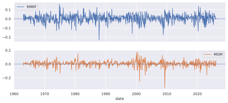

And the 7-year rolling average to assess the persistence of the momentum premium over time:

axes = mom.rolling(84).mean().plot(figsize=(12,5), subplots=True, sharey=True)
for c in axes:
    c.axhline(y=0, lw=1)
plt.show()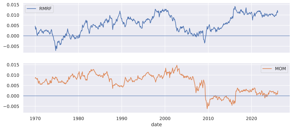

The rolling average reveals that the US momentum premium was strong and fairly stable through the 1990s and early 2000s, but has been notably weak, and at times negative, since around 2009. Part of this weakness comes from the momentum crash of 2009 studied by Daniel and Moskowitz (2016). They show that momentum crashes occur in panic states, following market declines and when market volatility is high, and coincide with market rebounds, when the past losers that momentum strategies sell short rally. From March to May 2009, the decile of past losers rose by 163% while the decile of past winners gained only 8%.

Daniel, Kent, and Tobias J. Moskowitz. 2016. “Momentum Crashes.” Journal of Financial Economics 122 (2): 221–47.

International Comparison

A natural question is whether the weakness of US momentum since 2009 is a global phenomenon or specific to the US market. Kenneth French’s data library provides momentum factors for international markets, allowing us to compare. We download the momentum factor for Europe and Emerging Markets using the same CarhartFactors class with the region argument. Note that for international factors the momentum column is named WML (Winners Minus Losers) rather than MOM.

europe = (CarhartFactors(frequency='m', region='europe', start_date=start_date)
          .load()
          .to_pandas()
          [['WML']]
          .rename(columns={'WML': 'Europe'})
          )

emerging = (CarhartFactors(frequency='m', region='emerging', start_date=start_date)
            .load()
            .to_pandas()
            [['WML']]
            .rename(columns={'WML': 'Emerging'})
            )

mom_intl = (mom[['MOM']]
            .rename(columns={'MOM': 'US'})
            .join([europe, emerging], how='inner')
            )

display(mom_intl)

	US	Europe	Emerging
date
1991-04-30	-0.0233	0.0156	0.0469
1991-05-31	-0.0010	-0.0064	0.0364
1991-06-30	0.0042	0.0054	0.0128
1991-07-31	0.0426	0.0506	0.0009
1991-08-31	0.0158	0.0377	-0.0015
...	...	...	...
2026-05-31	0.0139	0.0115	0.0958
2026-06-30	0.0462	0.0100	0.0036
2026-07-31	-0.1221	-0.0782	-0.1684
2026-08-31	-0.0560	-0.0071	0.0802
2026-09-30	0.0670	0.0606	0.0592

426 rows × 3 columns

Note that in the data we download, the European momentum series begins in April 1991 and the Emerging Markets series in January 1990, both much later than the US series, which we start in 1963 (Kenneth French’s US data go back to 1927). The inner join above restricts mom_intl to the period where all three series overlap, so the chart below covers a shorter sample than the US-only plots above.

We plot the 7-year rolling average for each region to compare the persistence of the momentum premium across markets:

ax = mom_intl.rolling(84).mean().plot(figsize=(12,5))
ax.axhline(y=0, lw=1)
ax.set_ylabel('Monthly Return')
plt.show()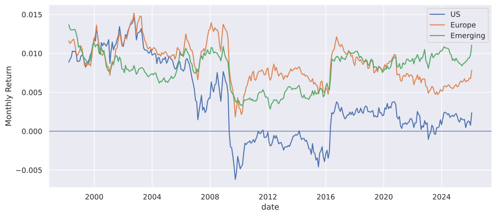

The graph shows that while the US momentum premium has weakened considerably since 2009, momentum in Europe has been more resilient and has remained positive for most of the sample period. Emerging Markets momentum is more volatile and its rolling average has fluctuated more widely, reflecting the greater macroeconomic uncertainty and lower market efficiency that characterize these economies. The fact that momentum persists across multiple geographically and institutionally distinct markets lends support to the view that it reflects a fundamental feature of investor behavior rather than a US-specific data artifact.

Practice Problems

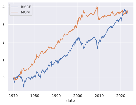
Problem 1 All factors are zero-cost portfolios, that is, they are long-short strategies in which the long position is exactly financed by the short position. Compute the cumulative sum of RMRF and MOM from January 1970 until May 2023.

Hint: For a given dataframe df, the function df.cumsum() computes the cumulative sum of all columns.

Solution

mom = (CarhartFactors(frequency='m', start_date='1970-01-01', end_date='2023-05-01')
       .load()
       .to_pandas()
       .rename(columns={'Mkt-RF': 'RMRF'})
       [['RMRF', 'MOM']]
       )

mom.cumsum().plot()
plt.show()

Note that the cumulative sum of monthly returns for both factors over the period is similar. The momentum factor accumulates more quickly at the beginning but trails off toward the end as the premium weakens.