The Capital Asset Pricing Model
Investment Theory
Fall 2026
From Beta Pricing to the CAPM
- Beta pricing holds for any mean-variance efficient portfolio Q: \operatorname{E}(r_{A}) = (1 - \beta_{A}) r_{f} + \beta_{A} \operatorname{E}(r_{Q}).
- It does not say which portfolio is efficient.
- Building Q directly needs \pmb{w}_{Q} \propto \pmb{\Sigma}^{-1}(\pmb{\mu} - r_{f}\mathbf{1}), and both inputs are hard to estimate.
- The CAPM supplies the missing link: in equilibrium, Q is the market portfolio M.
- Market weights need no estimates of expected returns or covariances.
- In practice, broad value-weighted indexes proxy for M.
The Assumptions
- Investors evaluate portfolios by their means and variances.
- They share the same expected returns and covariance matrix (homogeneous expectations).
- They trade the same assets without frictions and borrow or lend at a common risk-free rate.
- Markets clear.
Two-Fund Separation
- An investor with risk aversion A holds weight w^{*} = \frac{\mu_{Q} - r_{f}}{A \sigma_{Q}^{2}} in the tangency portfolio Q.
- With homogeneous expectations, every investor faces the same frontier and picks the same Q.
- More risk-averse investors lend and hold less of Q; less risk-averse investors borrow and hold more.
- Either way, they all hold the risky assets in Q’s proportions.
Two-Fund Separation in a Picture
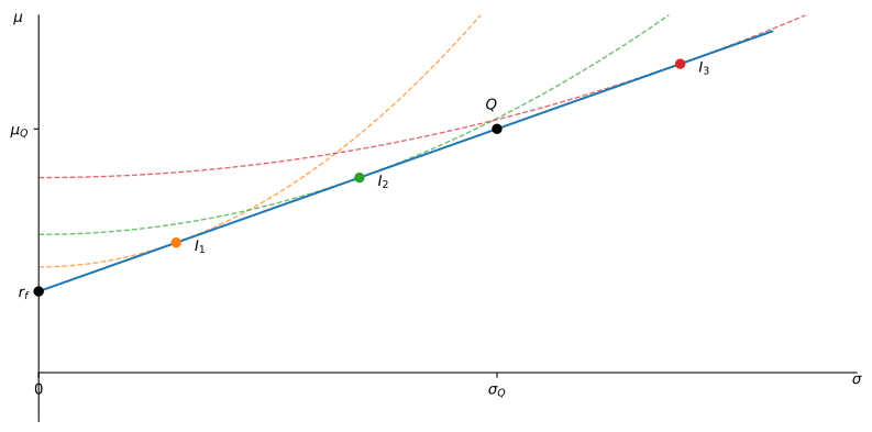
Figure 1: Three investors hold Q in different amounts, each at the point where an indifference curve (dashed) is tangent to the CAL.
Aggregation and Market Clearing
- Let q_{j} be asset j’s weight in Q and W_{i} investor i’s wealth. Aggregate demand for asset j is
q_{j} \sum_{i} w_{i}^{*} W_{i}.
- The sum is the same for every asset, so aggregate risky demand has Q’s composition.
- Market clearing: investors must hold the outstanding supply, whose weights are V_{j}/\sum_{k} V_{k}, the weights of the market portfolio M.
- Therefore Q = M.
- The conclusion concerns relative weights within the risky portfolio; the risk-free asset need not be in zero net supply.
When the Argument Fails
- If investors disagree about expected returns or covariances, face different borrowing rates, or cannot trade the same assets, they need not choose the same tangency portfolio.
- Two-fund separation then fails at the aggregate level.
- Market clearing no longer implies that M is mean-variance efficient.
Property 1 (The Capital Asset Pricing Model) If the assumptions of the CAPM hold, the market portfolio M is mean-variance efficient. Substituting Q = M into the beta pricing formula, the expected excess return of any asset A is proportional to its market beta: \operatorname{E}(r_{A}) - r_{f} = \beta_{A} \bigl[\operatorname{E}(r_{M}) - r_{f}\bigr], \tag{1} where \beta_{A} = \frac{\operatorname{Cov}(r_{A}, r_{M})}{\operatorname{V}(r_{M})}.
Reading the CAPM
- The market risk premium \operatorname{E}(r_{M}) - r_{f} is the expected return investors require for bearing one unit of market risk.
- An asset with \beta_{A} = 1 has the same expected excess return as the market; one with \beta_{A} < 1 has a smaller one.
- Expected returns are determined entirely by exposure to market risk.
- Idiosyncratic volatility does not enter because it can be diversified away.
Example 1 (Computing a Stock Beta) Suppose that the correlation between stock A and the market is 0.6. If the standard deviation of A returns is 40% per year, and the standard deviation of the market is 20% per year, the beta of A is \begin{aligned} \beta_{A} & = \frac{\operatorname{Cov}(r_{A}, r_{M})}{\operatorname{V}(r_{M})} = \frac{\sigma_{A} \sigma_{M} \rho_{A,M}}{\sigma_{M}^{2}} \\ & = \frac{\sigma_{A} \rho_{A,M}}{\sigma_{M}} = \frac{0.4 \times 0.6}{0.2} = 1.2. \end{aligned}
Example 2 (Computing an Expected Return) If the risk-free rate is 5%, \beta_{DELL} = 1.3, and \operatorname{E}(r_{M}) = 14\%, then the CAPM predicts that: \operatorname{E}(r_{DELL}) = 0.05 + 1.3 \times (0.14 - 0.05) = 16.7\%. The 16.7% is Dell’s expected annual total return, including both price changes and distributions such as dividends. It is an average required return, not a guarantee of the return that will be realized next year.
Systematic and Firm-Specific Risk
- Under the CAPM, the return of any asset can be decomposed into a systematic and a firm-specific part, r_{A} - r_{f} = \beta_{A} (r_{M} - r_{f}) + \varepsilon_{A}, \tag{2} where \operatorname{E}(\varepsilon_{A}) = 0 and \operatorname{Cov}(\varepsilon_{A}, r_{M}) = 0.
- Because the two parts are uncorrelated, the total variance splits as \sigma_{A}^{2} = \beta_{A}^{2} \sigma_{M}^{2} + \sigma^{2}(\varepsilon_{A}). \tag{3}
- Systematic variance \beta_{A}^{2} \sigma_{M}^{2} remains in a diversified portfolio; firm-specific variance \sigma^{2}(\varepsilon_{A}) can be diversified away.
- Only \beta_{A} determines expected return.
Example 3 (Computing the Residual Risk) Suppose that stock A has a standard deviation of returns of 40% per year and a market beta of 1.1. The standard deviation of the market return is 20%.
This means that the residual variance is \sigma^{2}(\varepsilon_{A}) = \sigma_{A}^{2} - \beta_{A}^{2} \sigma_{M}^{2} = 0.40^{2} - 1.1^{2} \times 0.20^{2} = 0.1116. Therefore, the standard deviation of the firm-specific risk is \sqrt{0.1116} = 33.41\%.
Interpreting Empirical Evidence
- The CAPM is a statement about expected returns, which cannot be observed directly.
- Realized returns vary around their expectations, so a stock can beat or miss the CAPM prediction in a given year without violating the model.
- Tests use many realized returns to estimate whether average returns line up with beta.
- A persistent deviation has several possible explanations:
- The asset is mispriced.
- The CAPM’s assumptions fail, so the market portfolio is not mean-variance efficient.
- The index used in the test is a poor proxy for the theoretical market portfolio, which cannot be observed (Roll, 1977).
The Joint-Hypothesis Problem
- Every empirical test of market efficiency is also a test of the asset-pricing model used to define the correct expected return.
- Rejecting the CAPM relation therefore rejects the combined hypothesis, not necessarily market efficiency alone.