Forward Rates
Investment Theory
Fall 2026
Computing Forward Rates
Synthesizing Forward Rates
- The term structure of interest rates allows investors to lock future interest rates using forward-rates that can be synthesized from zero-coupon rates.
- Denote by Z(n) the price of a zero-coupon bond with face value equal to $1 and expiring at year n.
- Consider now two zero-coupon bonds with expirations m < n, that we will denote by M and N, respectively.
- Suppose we sell \frac{Z(n)}{Z(m)} units of bond M and invest the proceeds in bond N.
- The proceeds from selling \frac{Z(n)}{Z(m)} units of M are the number of units times the price per unit, i.e., \frac{Z(n)}{Z(m)} \times Z(m) = Z(n).
- Therefore, by selling \frac{Z(n)}{Z(m)} units of M you get the amount needed to buy 1 unit of bond N.
Cash Flows from the Strategy
The table below shows that this strategy creates a forward-starting zero-coupon bond.
Year 0 m n Sell \frac{Z(n)}{Z(m)} units of M Z(n) -\frac{Z(n)}{Z(m)} 0 Buy 1 unit of N -Z(n) 0 1 Total 0 -\frac{Z(n)}{Z(m)} 1 Instead of investing a certain amount today at a known interest rate, and therefore guaranteeing a known amount at maturity, this newly created security guarantees today that if you invest a certain amount in year m, you will earn a known interest rate from year m to year n.
The Forward Rate
- The implicit annualized interest rate f(m, n) that applies to this newly created security is called the forward-rate from year m to n, which must satisfy \frac{1}{(1 + f(m, n))^{(n - m)}} = \frac{Z(n)}{Z(m)}, so that f(m, n) = \left( \frac{Z(m)}{Z(n)} \right)^{\!\frac{1}{n - m}} - 1. \tag{1}
Example 1 (Computing Forward Rates) Given
| Bond | Maturity (years) | Price ($) |
|---|---|---|
| Z_{1} | 1 | 920 |
| Z_{2} | 2 | 840 |
| Z_{3} | 3 | 760 |
| Z_{4} | 4 | 710 |
\begin{aligned} f(2, 4) & = \left(\frac{840}{710}\right)^{\!1/2} - 1 = 8.77\%, \\ f(1, 4) & = \left(\frac{920}{710}\right)^{\!1/3} - 1 = 9.02\%, \\ f(3, 4) & = \frac{760}{710} - 1 = 7.04\%. \end{aligned}
Forward and Zero-Coupon Rates
- Sometimes, the forward rate is expressed as a function of the zero-coupon rates implicit in the zero-coupon bond prices.
- If we denote by r(m) and r(n) the zero-coupon rates corresponding to maturities m and n, respectively, 1 can be re-written as f(m, n) = \left( \frac{(1 + r(n))^{n}}{(1 + r(m))^{m}} \right)^{\!\frac{1}{n - m}} - 1. \tag{2}
Intuition
- Note that if we could fix the forward rate f(m, n) beforehand, then it must be the case that investing from 0 to m at r(m), and then rolling the deposit from m to n at f(m, n), should be equivalent to investing all the way from 0 to n at r(n).
- If not, there would be a simple arbitrage opportunity where we could invest using the strategy that delivers the most and borrow using the other alternative.
- Therefore, it must be the case that: (1 + r(m))^{m} (1 + f(m, n))^{n - m} = (1 + r(n))^{n}, which also delivers (2).
Example 2 (One-Year Forward Rates) The table below shows the zero-coupon rate per year compounded annually for different maturities. The forward rate that applies from the previous to the current year is computed in the last column.
| Year | Zero Rate (%) | Forward Rate (%) |
|---|---|---|
| 1 | 4.0 | |
| 2 | 5.0 | 6.01 |
| 3 | 5.6 | 6.81 |
| 4 | 6.0 | 7.21 |
| 5 | 6.3 | 7.51 |
In the table, the forward rate that applies from year 1 to 2 is computed as f(1, 2) = \frac{1.05^{2}}{1.04} - 1 = 6.01\%, whereas the forward rate that applies from year 4 to 5 is given by f(4, 5) = \frac{1.063^{5}}{1.06^{4}} - 1 = 7.51\%.
Forward Rates and the Yield Curve
Forward Rates with Continuous Compounding
- With continuously compounded zero yields y_{t}(n), as in Bond Pricing, f_{t}(m, n) = \frac{n \, y_{t}(n) - m \, y_{t}(m)}{n - m}.
- The yield to maturity n is the average of the forward rates over the life of the bond: y_{t}(n) = \frac{1}{n} \sum_{k=0}^{n-1} f_{t}(k, k+1), \qquad f_{t}(0, 1) = y_{t}(1).
- An upward-sloping yield curve has a forward curve above it; a downward-sloping one, below it.
The Forward Curve
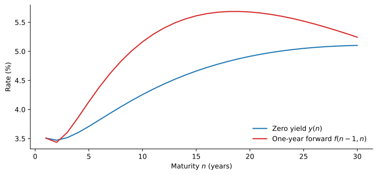
Continuously compounded zero yields and one-year forward rates on December 31, 2025, from the Treasury curve of Gürkaynak et al. (2007).
- The one-year rate was 3.51%, the forward for year 10 was 5.16%, and the forwards peaked near 5.7%.
Term Premia
Forward Rates and Expected Rates
- A forward rate can be locked in today. Is it also a forecast of the future rate?
- Write it as the expected one-year rate plus a term premium: f_{t}(n - 1, n) = \operatorname{E}_{t}\left( y_{t + n - 1}(1) \right) + \mathit{TP}_{t}(n).
- The term premium is whatever separates the forward rate from the expected rate, apart from a small convexity effect.
The Term Premium Is an Expected Excess Return
- Buy a 2-year zero and sell it after a year. Its log return in excess of the one-year yield is \mathit{rx}_{t+1}(2) = 2 y_{t}(2) - y_{t}(1) - y_{t+1}(1) = f_{t}(1, 2) - y_{t+1}(1).
- The bond beats the one-year deposit when next year’s rate turns out below today’s forward rate.
- Taking expectations: \operatorname{E}_{t}(\mathit{rx}_{t+1}(2)) = \mathit{TP}_{t}(2).
- A positive term premium compensates for holding a bond whose price falls when rates rise.
Three Theories, One Question
- The traditional theories of the term structure are statements about \mathit{TP}_{t}(n):
- Expectations hypothesis: zero, so forward rates are expected short rates.
- Liquidity preference: positive and rising with maturity.
- Segmented markets: set by supply and demand at each maturity.
- Which fits the data is an empirical question: The Term Structure in the Data.
The Expectations Hypothesis
- Risk-neutral investors: every bond has the same expected return over the next year, the one-year rate.
- For a bond with annual coupons C: \operatorname{E}(R_{1}) = \frac{\operatorname{E}(B_{1}) + C}{B_{0}} - 1 = r_{0}(1).
- An upward-sloping curve means short rates are expected to rise; a downward-sloping one, to fall.
- Short rates rise about as often as they fall, so under the EH the curve should be flat on average.
Example 3 (Computing an Expected Bond Price) Suppose you have the following information on zero-coupon rates.
| Maturity (years) | Rate (%) |
|---|---|
| 1 | 5.0% |
| 2 | 5.5% |
| 3 | 6.0% |
| 4 | 6.3% |
| 5 | 6.5% |
Consider a 4% annual-paying coupon bond over a notional of $1,000 expiring in 5 years. The price of this bond today can be computed by discounting its cash flows at the appropriate zero-rate. B_{0} = \frac{40}{1.05} + \frac{40}{1.055^{2}} + \frac{40}{1.06^{3}} + \frac{40}{1.063^{4}} + \frac{1040}{1.065^{5}} = 898.02
If the EH holds, the price of this bond next year, B_{1}, should be such that \frac{B_{1} + C}{B_{0}} = 1 + r_{0}(1), implying B_{1} = 898.02 \times 1.05 - 40 = \$902.92.
The Curve Is Not Flat on Average
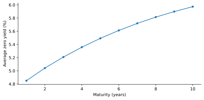
Average continuously compounded zero-coupon Treasury yield by maturity, month-end, 1972 to 2025.
- The 1-year yield started at 4.2% and ended at 3.5%, yet the 10-year yield was above it in 81% of the months: a positive average term premium.
The Liquidity Preference Theory
- The EH treats bonds of all maturities as perfect substitutes.
- Risk-averse investors care about the volatility of rates too:
- Long-term bondholders face price risk if they sell before maturity, and want compensation.
- Issuers are willing to pay more to lock in a rate for many years.
- The term premium is positive and grows with maturity, so the curve slopes up on average: r_{0}(2) > \frac{r_{0}(1) + \operatorname{E}(r_{1}(1))}{2}.
Segmented Markets and Preferred Habitat
- Segmented markets: investors do not substitute across maturities.
- Money market funds hold short bonds; pension funds and insurers, matching long liabilities, hold long ones.
- Each segment’s rate is set by its own supply and demand.
- Preferred habitat: investors leave their preferred maturities for a high enough premium.
- The term premium at each maturity depends on supply relative to demand.
- It changes when the Treasury changes the maturity of its debt, or the Federal Reserve buys long bonds.
The Convexity Adjustment
- Even under the EH, forward rates are not exactly expected rates, because bond prices are convex in yields.
- If expected discount factors equal forward discount factors, Jensen’s inequality gives \operatorname{E}(r_{t}(n)) > f(t, t + n).
- A second-order approximation shows the gap is small:
\frac{1 + \mu}{1 + f} \approx \left(1 + \frac{1}{2} n (n + 1) \left(\frac{\sigma}{1 + \mu}\right)^{\!2} \right)^{\!1/n},
where \mu = \operatorname{E}(r_{t}(n)) and \sigma^{2} = \operatorname{V}(r_{t}(n)).
- About 3 basis points for 5 years with \sigma = 1\%, about 21 for 10 years with \sigma = 2\%.