Stablecoins and Peg Risk

Introduction

Stablecoins are crypto tokens meant to keep a fixed price, usually about $1. They are widely used in crypto markets for trading, collateral, payments, and moving liquidity between platforms. But they are not risk-free. A stablecoin stays near its peg only if its reserves are trustworthy, redemptions work smoothly, and users remain confident. If any of these weaken, the token can trade below $1, causing losses and broader market stress.

Economically, a stablecoin is a short-term liability backed by a redemption promise. The main issue is whether investors trust that promise during periods of stress. This notebook examines that question with basic data checks and simple models. The objective is to explain why pegs break and what those moves signal about risk. Rather than random fluctuations, depegs often reflect market pricing of redemption risk and liquidity risk, which can reveal the system’s underlying health.

Three Economic Designs

The term stablecoin covers multiple economic designs. In all cases, the peg objective is similar, but the mechanism is different.

Fiat-backed (custodial) design. The issuer holds off-chain reserve assets (such as cash, bank deposits, and short-term Treasury instruments) and offers redemption at or near par. The peg mechanism is straightforward: if market price falls below $1, traders buy the coin and redeem with the issuer; if price rises above $1, they can mint or source supply and sell into the market. In practice, peg quality depends on reserve transparency, legal claim structure, banking access, and operational redemption frictions. Even with high-quality reserves, delays, fees, or uncertainty about access can widen short-run deviations. Major examples include USDT (Tether) and USDC (Circle), both of which rely on custodial reserve management and off-chain redemption rails.

Crypto-collateralized design. The token is backed by on-chain assets posted in smart contracts, typically with over-collateralization requirements. Users lock collateral to mint the stablecoin, and positions are liquidated if collateral values fall below required thresholds. This design is more transparent on-chain, but peg stability depends on collateral quality, liquidation speed, oracle reliability, and protocol governance. During sharp market moves, falling collateral values and crowded liquidations can create stress, especially if market liquidity is thin. The canonical example is DAI (MakerDAO), which is minted against crypto collateral and stabilized through collateral ratios, liquidation rules, and governance parameters.

Algorithmic design. The protocol targets the peg primarily through supply adjustments and arbitrage incentives rather than fully reserved backing. A common approach is mint-burn conversion between the stablecoin and a secondary token, aiming to make deviations from $1 profitable to arbitrage away. These mechanisms can appear effective in calm conditions, but they rely heavily on continued demand and confidence in the broader system. If confidence falls, the stabilizing loop can reverse: arbitrage incentives weaken, selling pressure rises, and a self-reinforcing depeg can emerge quickly. The most prominent case is TerraUSD (UST), whose 2022 collapse illustrates how quickly an algorithmic peg can fail when confidence in the companion token mechanism breaks.

A compact valuation identity is: P_t = 1 - \lambda_t, where P_t is stablecoin price and \lambda_t is the market-implied discount for redemption/liquidity risk. A persistent depeg is therefore a risk premium, not just random noise. This interpretation is consistent with evidence that peg deviations reflect leverage, liquidity, and balance-sheet constraints rather than pure tracking noise (Gorton et al. 2026).

Data: Measuring Peg Deviations

We begin with daily prices for three major stablecoins and two large crypto assets for context.

import numpy as np
import pandas as pd
import matplotlib.pyplot as plt
import yfinance as yf

import warnings
warnings.simplefilter(action="ignore", category=FutureWarning)

tickers = ["USDT-USD", "USDC-USD", "DAI-USD", "BTC-USD", "ETH-USD"]
px = (
    yf.download(tickers, start="2021-01-01", progress=False)["Close"]
    .dropna(how="all")
)

px.tail()

Ticker	BTC-USD	DAI-USD	ETH-USD	USDC-USD	USDT-USD
Date
2026-02-11	66991.968750	0.999768	1940.621338	0.999903	0.999290
2026-02-12	66221.843750	0.999696	1946.940674	0.999868	0.999164
2026-02-13	68857.843750	1.000027	2048.527344	0.999987	0.999455
2026-02-14	69767.625000	0.999913	2086.009766	1.000021	0.999592
2026-02-15	68851.726562	0.999792	1961.853638	1.000005	0.999442

Our main variable is depeg distance: d_{i,t} = P_{i,t} - 1, which is positive when a token trades above $1 and negative when it trades below $1.

stables = ["USDT-USD", "USDC-USD", "DAI-USD"]
d = px[stables] - 1.0

summary = pd.DataFrame({
    "mean_depeg": d.mean(),
    "std_depeg": d.std(),
    "min_depeg": d.min(),
    "max_depeg": d.max(),
    "mean_abs_depeg": d.abs().mean(),
})
summary

	mean_depeg	std_depeg	min_depeg	max_depeg	mean_abs_depeg
Ticker
USDT-USD	0.000123	0.000723	-0.004128	0.011530	0.000454
USDC-USD	-0.000004	0.000787	-0.028500	0.010496	0.000198
DAI-USD	0.000077	0.001136	-0.026131	0.010310	0.000485

fig, ax = plt.subplots(figsize=(10, 5))
for c in stables:
    ax.plot(d.index, d[c], lw=1.2, label=c.replace("-USD", ""))
ax.axhline(0.0, color="black", lw=1, alpha=0.6)
ax.set(title="Daily Depeg Distance (Price - 1)", ylabel="Depeg Distance")
ax.legend()
ax.grid(alpha=0.3)
plt.tight_layout()
plt.show()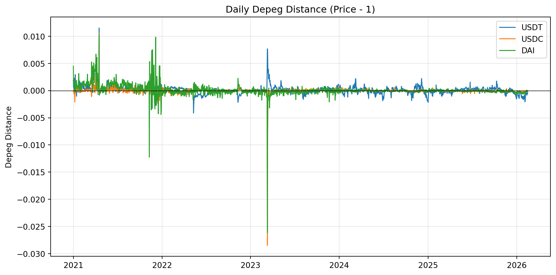

Arbitrage Logic Around the Peg

If redemption is smooth and cheap, price should stay close to $1. Let \kappa denote round-trip arbitrage cost, including fees, bid-ask spread, transfer delays, and balance-sheet costs. A simple no-arbitrage condition is: |P_t - 1| \leq \kappa in normal conditions.

If depeg distance often exceeds this band, markets are signaling friction. Likely causes include limited redemption capacity, inventory constraints, settlement delays, or concern about reserve quality. This is why depeg dynamics should be read as part of broader market liquidity and flow conditions, not only as coin-specific noise (Griffin and Shams 2020; Gorton et al. 2026).

kappa = 0.002  # 20 bps stylized friction band
band_exceed = (d.abs() > kappa).mean().rename("share_outside_band")
band_exceed

Ticker
USDT-USD    0.014957
USDC-USD    0.005876
DAI-USD     0.034188
Name: share_outside_band, dtype: float64

Run Risk as a Coordination Problem

Run risk is nonlinear because confidence can reinforce itself. If many holders redeem at once, liquidity pressure can force asset sales, weaken effective backing, and trigger more redemptions.

One reduced-form model for one-period run probability is: \Pr(\text{run}) = \sigma\!\left(a + b(1-c) + \gamma\,\ell\right), Here, c is collateral quality, \ell is leverage or liquidity mismatch, and \sigma(x)=1/(1+e^{-x}) is the logistic function. The key insight is that deterioration in collateral or liquidity can raise instability sharply once confidence drops past a threshold (Gorton et al. 2026).

Gorton, Gary B., Elizabeth C. Klee, Chase P. Ross, Sharon Y. Ross, and Alexandros P. Vardoulakis. 2026. “Leverage and Stablecoin Pegs.” Journal of Financial and Quantitative Analysis 61 (1): 99–136. https://doi.org/10.1017/S0022109025000134.

def logistic(x):
    return 1 / (1 + np.exp(-x))

a = -4.0
b = 5.0
gamma = 3.5

collateral_quality = np.linspace(0.70, 1.00, 7)
liquidity_mismatch = np.array([0.05, 0.10, 0.20, 0.30])

rows = []
for c in collateral_quality:
    for ell in liquidity_mismatch:
        p_run = logistic(a + b * (1 - c) + gamma * ell)
        rows.append({"collateral_quality": c, "liquidity_mismatch": ell, "run_prob": p_run})

run_table = pd.DataFrame(rows)
run_table.head()

	collateral_quality	liquidity_mismatch	run_prob
0	0.70	0.05	0.089074
1	0.70	0.10	0.104331
2	0.70	0.20	0.141851
3	0.70	0.30	0.190002
4	0.75	0.05	0.070765

fig, ax = plt.subplots(figsize=(8, 5))
for ell in liquidity_mismatch:
    sub = run_table[run_table["liquidity_mismatch"] == ell]
    ax.plot(sub["collateral_quality"], sub["run_prob"], marker="o", label=f"mismatch={ell:.2f}")

ax.set(
    title="Stylized Run Probability",
    xlabel="Collateral Quality",
    ylabel="Run Probability",
)
ax.grid(alpha=0.3)
ax.legend()
plt.tight_layout()
plt.show()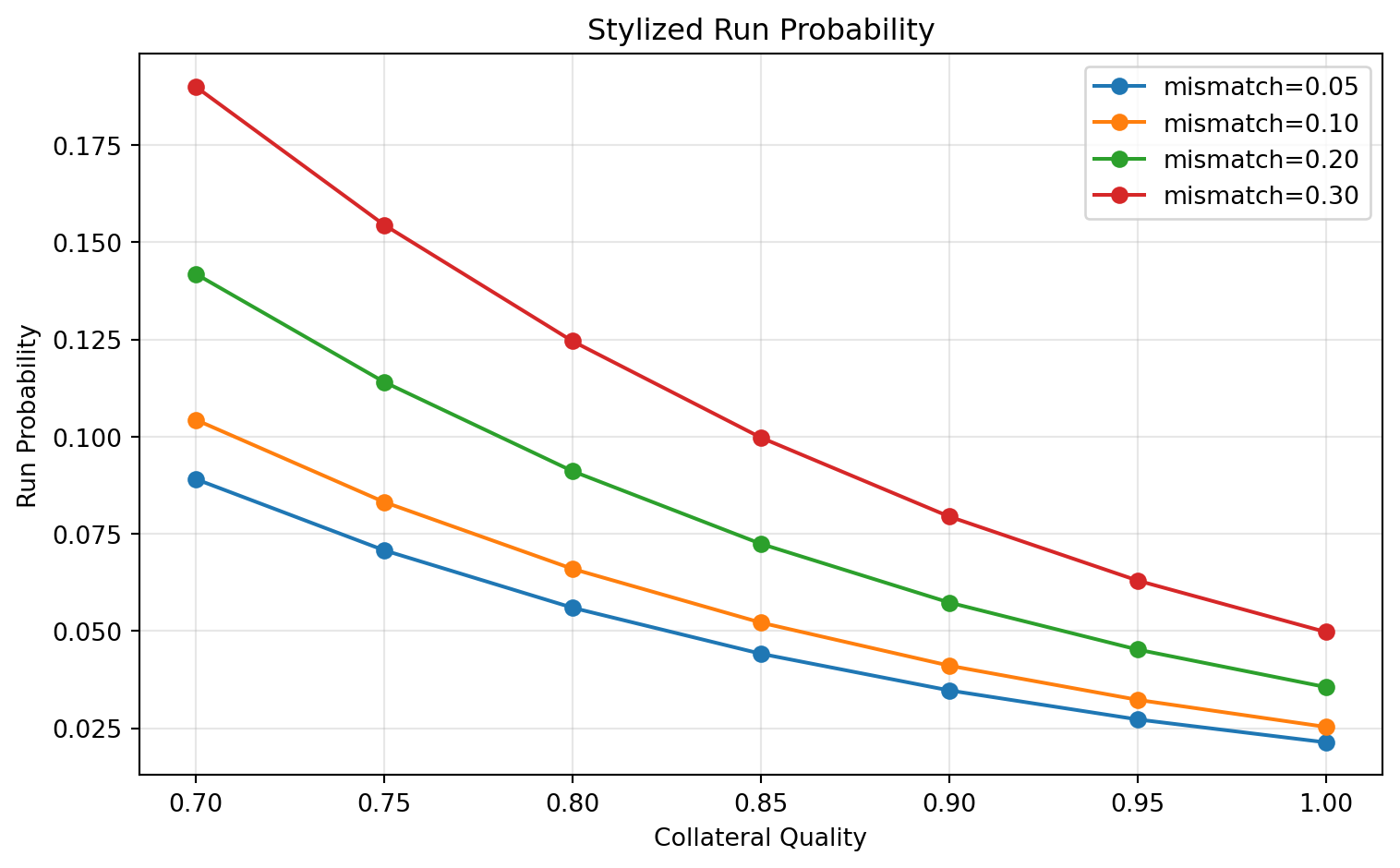

The simulation delivers clear comparative statics. Higher collateral quality lowers run probability, and larger liquidity mismatch raises it. The curve is nonlinear, so risk can increase quickly after confidence passes a critical point.

Stablecoins and Market Stress

Stablecoin depegs often move with broader crypto stress. A simple diagnostic is to compare average absolute depeg pressure with realized volatility in major crypto assets. This co-movement is consistent with evidence that stablecoin flows and crypto prices interact through demand and liquidity channels (Griffin and Shams 2020).

Griffin, John M., and Amin Shams. 2020. “Is Bitcoin Really Untethered?” Journal of Finance 75 (4): 1913–64. https://doi.org/10.1111/jofi.12903.

risk = px[["BTC-USD", "ETH-USD"]].pct_change().dropna()
rv = risk.rolling(30).std().mean(axis=1).rename("crypto_risk_30d")

depeg_pressure = d.abs().mean(axis=1).rename("avg_abs_depeg")
joined = pd.concat([rv, depeg_pressure], axis=1).dropna()
joined.corr()

/tmp/ipykernel_1705315/2812493833.py:5: Pandas4Warning: Sorting by default when concatenating all DatetimeIndex is deprecated.  In the future, pandas will respect the default of `sort=False`. Specify `sort=True` or `sort=False` to silence this message. If you see this warnings when not directly calling concat, report a bug to pandas.
  joined = pd.concat([rv, depeg_pressure], axis=1).dropna()

	crypto_risk_30d	avg_abs_depeg
crypto_risk_30d	1.000000	0.150912
avg_abs_depeg	0.150912	1.000000

fig, ax = plt.subplots(figsize=(8, 5))
ax.scatter(joined["crypto_risk_30d"], joined["avg_abs_depeg"], s=10, alpha=0.6)
ax.set(
    title="Depeg Pressure vs 30-Day Crypto Volatility",
    xlabel="30-day realized volatility (BTC/ETH average)",
    ylabel="Average absolute depeg",
)
ax.grid(alpha=0.3)
plt.tight_layout()
plt.show()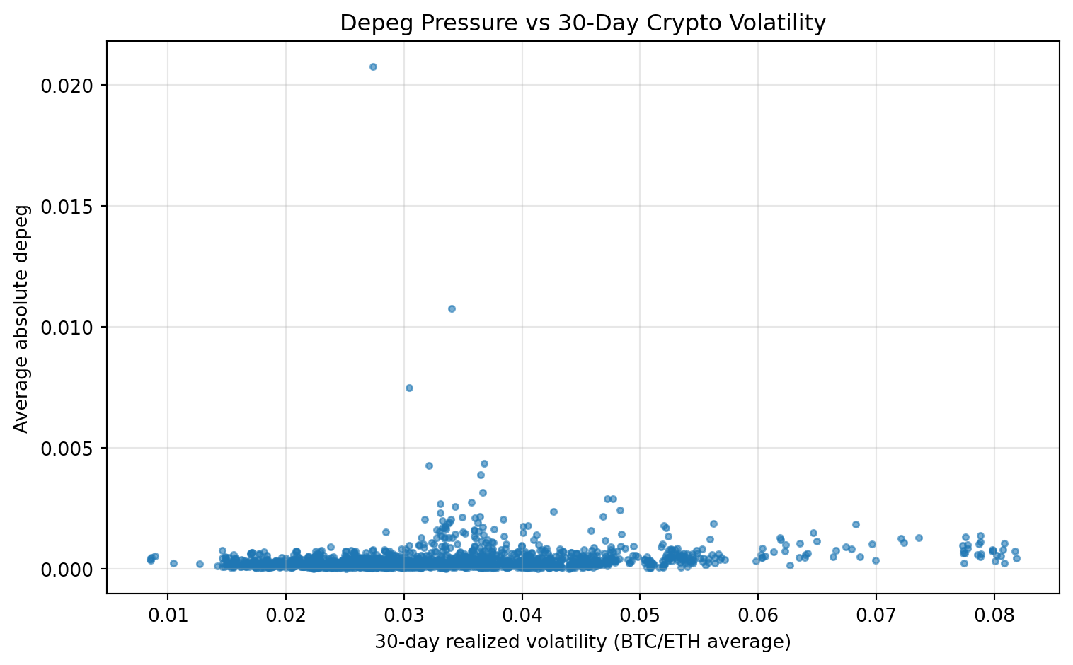

This relationship is descriptive, not causal. Still, it matches the intuition that balance-sheet and liquidity constraints bind more tightly when volatility is high.

Takeaways

Stablecoin economics can be summarized with three questions. What assets back the liability, and how quickly can they be sold at par? How does redemption work, and who can access it during stress? How strong are governance and risk controls when markets are volatile?

For empirical analysis, small and persistent deviations from $1 are informative. They measure market-implied redemption and liquidity risk, and they help separate normal arbitrage frictions from deeper solvency concerns.