Automated market makers (AMMs) are pricing and execution mechanisms used inside many crypto exchanges. Instead of matching buyers and sellers in a limit-order book, an AMM pool sets prices with explicit formulas and pooled liquidity, so execution and price adjustment are rule-based (Adams et al. 2020).
In plain terms, on a decentralized exchange (DEX) such as Uniswap, an AMM pool is a smart-contract system that holds token reserves and automatically quotes a swap rate from a formula. A trader does not need a matching counterparty at that moment; the counterparty is the pool itself. The trade updates reserves, and the formula immediately updates the next quote.
Here a smart contract means executable code deployed at an on-chain address.1 When users submit transactions, blockchain validators execute that code and update state (for example reserves, liquidity positions, and fees) according to pre-specified rules. So the exchange logic runs on-chain, while web apps are mainly interfaces that help users send those transactions.
1 An on-chain address can refer either to a user wallet account (controlled by a private key) or to a contract account (which contains code and state). AMM pools are contract accounts, while traders and LPs typically interact from wallet accounts.
At a high level, a DEX such as Uniswap is a rules-based system of on-chain contracts rather than a single centralized exchange company running an internal account ledger. This system coordinates four main participant roles: traders (who swap), liquidity providers (LPs, who supply inventory and earn fees), arbitrageurs (who align pool prices with broader markets), and developers/frontends (who build access layers and tools).
One useful analogy is to view a DEX with AMM pools as an automated trading desk. The quote engine is a formula in a smart contract, not a human dealer, and the inventory behind those quotes is capital supplied by LPs. LPs can choose different fee-earning styles by choosing different pools, fee tiers, and (in v3/v4) active price ranges. This is close in spirit to traditional OTC markets, where liquidity is dealer-intermediated rather than matched in one centralized order book.2
2 Operationally, becoming an LP means depositing tokens into one of these pool contracts. In a v2-style pool, the LP deposits both assets in the pool ratio and receives a pro-rata claim on the pool and its fees. In v3/v4-style pools, the LP also chooses a price range for active liquidity, so fee earning depends on whether trading occurs inside that chosen range.
Market Structure and Motivation
Many decentralized exchanges (DEXs), such as Uniswap, Curve, and Balancer, use AMM pools as their execution mechanism. By contrast, most centralized exchanges (CEXs), such as Coinbase, Binance, and Kraken, rely on traditional CLOB-style matching.3
3 In this sense, DEX trading is not a completely new economic idea: it resembles currency trading in decentralized OTC markets, but with execution rules encoded on-chain.
This distinction is different from traditional equity market structure. In stock markets, exchanges (for example, NYSE or Nasdaq) mainly provide matching and price discovery, while custody is handled by brokers and custodians. Many crypto CEXs combine these roles: they operate the trading venue and also act as broker-custodian for client assets.
That institutional bundling matters for investor protection and market conduct. In U.S. equity markets, brokers and exchanges operate under established SEC and FINRA frameworks with clearer supervision and enforcement. In crypto, protections vary substantially across jurisdictions and platforms, and weaker oversight can increase exposure to freezes, bankruptcy disputes, or unilateral account actions.
A related microstructure concern is informational conflict: because a CEX can observe customer orders in real time, it can in principle trade against that flow (or advantage affiliates) unless governance, surveillance, and regulation constrain such behavior.
NoteWhy DEX Design Can Help: Documented CEX Conflict Cases
Several documented cases motivate the focus on transparent, rule-based on-chain trading:
Binance CFTC case (documented allegations and settlement): The March 27, 2023 CFTC complaint alleged proprietary trading and conflicts; the main resolution/settlement with Binance (and CZ) across agencies (CFTC, DOJ, FinCEN, OFAC) happened on November 21, 2023, with the court formally entering the CFTC consent order on December 18, 2023.
Complaint: https://www.cftc.gov/media/8351/enfbinancecomplaint032723/download
Settlement: https://www.cftc.gov/PressRoom/PressReleases/8837-23
These outcomes were possible largely because U.S. regulators and courts had jurisdiction and could enforce rules. In offshore or weakly supervised jurisdictions, comparable enforcement can be slower, narrower, or practically unavailable.
DEXs do not eliminate all risks, but they reduce some informational asymmetries by making execution rules and state transitions publicly auditable on-chain.
For this class, DEXs are a useful laboratory because pricing rules, liquidity state, and transaction-level outcomes are directly observable on-chain. Even when CEXs dominate aggregate volume, DEX data provide a cleaner setting to study core microstructure concepts that are also central in OTC currency markets: price impact, arbitrage transmission, fee formation, and inventory risk.4
4 Traditional OTC markets also use automated, inventory-sensitive quoting, so the economic logic is not entirely new. What is distinctive in crypto AMMs is the architecture: explicit formula-based pricing, always-on pooled liquidity, and publicly auditable state transitions, which makes them unusually accessible for empirical microstructure analysis.
This notebook studies AMM mechanics with simple models and data simulations. For pedagogical clarity, we use the Uniswap v2-style full-range constant-product framework as a baseline before discussing richer designs such as concentrated liquidity in v3 and programmable hooks in v4 (Uniswap Labs 2025; Adams et al. 2024). We focus on five questions. How does constant-product pricing work? How does trade size create slippage? How do arbitrageurs realign AMM prices with external markets? How do liquidity providers (LPs) earn fees? When do LPs lose value through impermanent loss?
Terminology used in this note: Uniswap is the DEX protocol (venue and rules), while the AMM pool is the pricing mechanism traders interact with inside that protocol.
Constant-Product Pricing
A standard AMM pool holds reserves of two assets, x and y, and enforces
x y = k.
In practice, x and y are tokens on the same blockchain, for example ETH and USDC or two stablecoins.5 A useful economic interpretation is that most crypto tokens are valued primarily by exchange demand, network use, and relative scarcity, not by direct claims on physical assets or contractual cash flows. That makes AMM trading naturally a currency-pair problem: each token’s value is quoted relative to another token, just as in FX markets (for example, EUR/USD).
5 AMM swaps settle atomically inside one contract execution. For that, the pool contract must be able to transfer both assets under the same chain’s state rules. Cross-chain swaps require additional bridge or messaging layers and introduce extra latency and risk.
Adams, Hayden, Noah Zinsmeister, Moody Salem, River Keefer, and Dan Robinson. 2020. Uniswap V2 Core. Uniswap Whitepaper. https://docs.uniswap.org/whitepaper.pdf.
Under this view, an AMM pool is a two-currency dealer balance sheet. The ratio y/x is an exchange rate, and swaps are conversions between two monetary units. The constant k is the pool’s invariant: it does not change except when LPs add or remove liquidity. In Uniswap-style AMMs, this invariant provides a transparent, auditable pricing rule on-chain (Adams et al. 2020). When a trader buys asset x by selling asset y, the pool’s x reserve shrinks and its y reserve grows. The product k stays fixed, which automatically raises the price of the remaining x and lowers the price of y. This algebra replaces discrete order-book matching with a continuous pricing curve. The missing x does not disappear: it is transferred out of the pool to the trader’s wallet, while the trader’s y is transferred into the pool. For a small swap, define the marginal exchange rate as
P=\frac{y}{x}.
This is the same convention used in currency markets: P is the x/y quote, meaning “units of y per one unit of x.” For example, if x= EUR and y= USD, then P is the EUR/USD quote (USD per EUR).
If a trader buys x from the pool, x reserves fall and y reserves rise. The ratio y/x increases, so the effective price moves against the trader. This is the core source of endogenous price impact in AMMs.
Mapping to Traditional Market Microstructure
The closest traditional analog to a constant-product AMM is a dealer that commits to an inventory-based quoting rule. This resembles OTC FX markets, where currency pairs trade across decentralized dealer networks rather than through one consolidated order book. In a central limit order book (CLOB), depth appears as discrete limit orders at different prices. In an AMM, depth is encoded by the continuous curve xy=k.
This creates a direct parallel:
In a CLOB, a market buy order “walks the book” and consumes higher ask levels.
In an AMM, a buy order moves the pool along the curve and raises the marginal price y/x.
Both mechanisms imply the same empirical pattern: larger trades relative to available depth generate larger price impact.
Execution costs also map cleanly across market designs:
CLOB taker cost: bid-ask spread + market impact.
AMM taker cost: swap fee + curve slippage.
Liquidity provider (LP) economics also mirror dealer economics. LPs earn fee income for supplying liquidity, but they bear inventory risk when prices trend. In AMMs this appears as impermanent loss, which is closely related to inventory and adverse-selection costs in traditional market making, including dealer-style currency markets.
Quick Numerical Analogy
Suppose a pool starts at x_0=y_0=1{,}000, so initial price is P_0=y_0/x_0=1. A trader sells \Delta y=100 into the pool to buy x:
So the trader receives about 90.91 units of x, paying an average price
P_{\text{avg}}=\frac{100}{90.91}\approx 1.10,
while the post-trade marginal price becomes
P_1=\frac{1{,}100}{909.09}\approx 1.21.
This is the AMM version of walking the ask side of an order book: average execution is worse than the pre-trade quote, and marginal price moves further against the next unit traded.
import numpy as npimport pandas as pdimport matplotlib.pyplot as pltx0 =1_000.0y0 =1_000.0k = x0 * y0def cp_swap_buy_x(delta_y, x=x0, y=y0):"""Trader adds delta_y of y to buy x from pool (no fees).""" y_new = y + delta_y x_new = k / y_new dx_out = x - x_new avg_price = delta_y / dx_out m_price_before = y / x m_price_after = y_new / x_newreturn {"delta_y_in": delta_y,"x_out": dx_out,"avg_price": avg_price,"marginal_before": m_price_before,"marginal_after": m_price_after, }trades = pd.DataFrame([cp_swap_buy_x(dy) for dy in [10, 50, 100, 200, 400]])show_table( trades.rename( columns={"delta_y_in": "Trade Size (y In)","x_out": "Asset x Received","avg_price": "Average Execution Price","marginal_before": "Marginal Price (Before)","marginal_after": "Marginal Price (After)", } ),4,)
Trade Size (y In)
Asset x Received
Average Execution Price
Marginal Price (Before)
Marginal Price (After)
10
9.9010
1.01
1.0
1.0201
50
47.6190
1.05
1.0
1.1025
100
90.9091
1.10
1.0
1.2100
200
166.6667
1.20
1.0
1.4400
400
285.7143
1.40
1.0
1.9600
In the table above, Asset x Received is the pure no-fee curve output implied by the invariant (x-x_{\text{new}}). Production DEX interfaces often display amount-out net of swap fees, so realized output there is typically lower than this teaching benchmark.
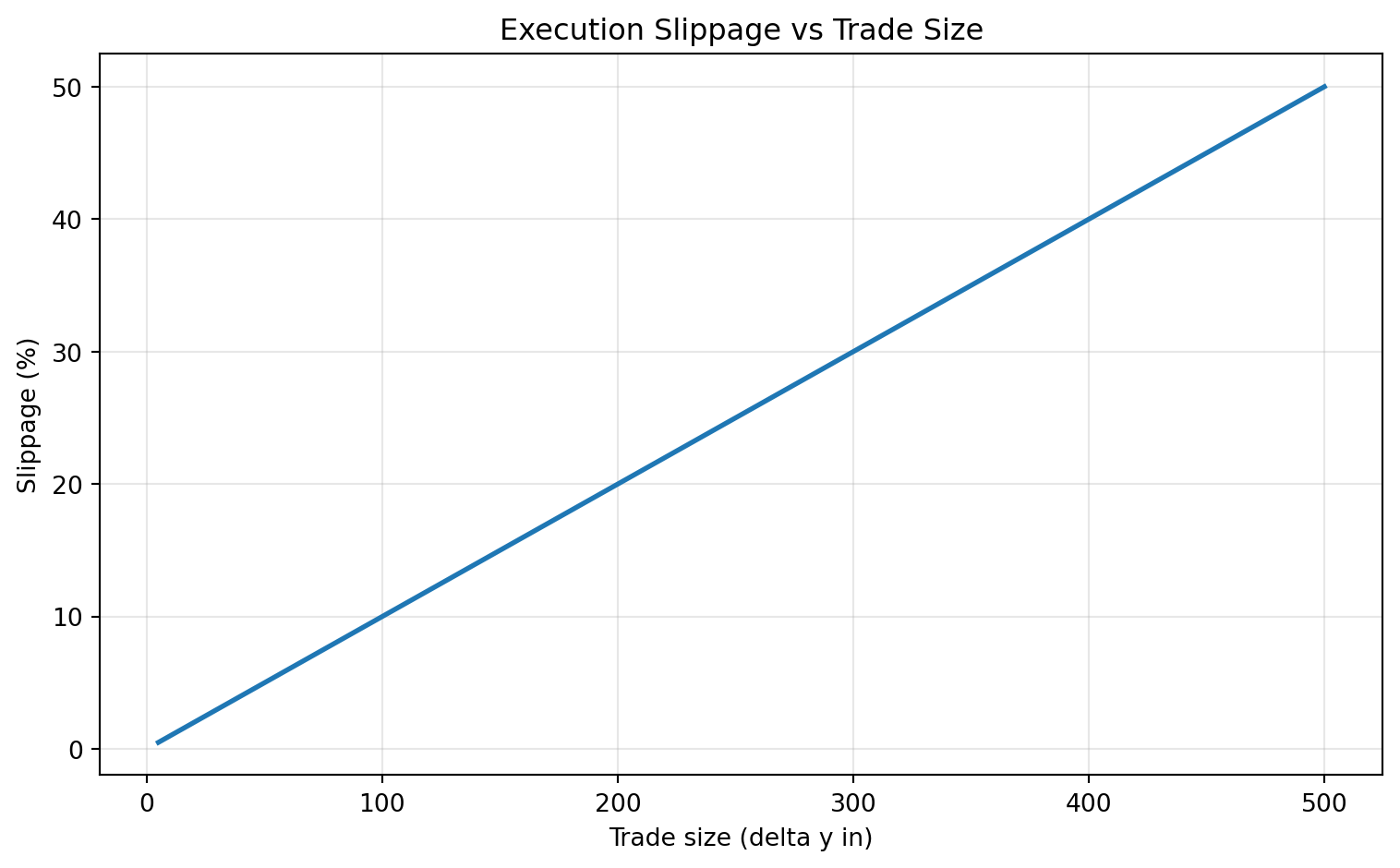
Slippage and Trade Size
In AMMs, slippage is the gap between the average execution price and the pre-trade marginal price. With constant-product pools, slippage grows with trade size relative to pool depth, just as market impact rises when a large order walks a thin CLOB.
A convenient metric is
\text{slippage} = \frac{P_{\text{avg}}}{P_{\text{pre}}}-1.
In deep pools, a given trade has low slippage. In shallow pools, the same trade can move price a lot.
pre_price = y0 / x0sizes = np.linspace(5, 500, 60)slip = []for dy in sizes: out = cp_swap_buy_x(dy) slip.append(out["avg_price"] / pre_price -1)slip = pd.Series(slip, index=sizes, name="slippage")slip.head()
fig, ax = plt.subplots(figsize=(8, 5))ax.plot(slip.index, 100* slip.values, lw=2)ax.set( title="Execution Slippage vs Trade Size", xlabel="Trade size (delta y in)", ylabel="Slippage (%)",)ax.grid(alpha=0.3)plt.tight_layout()plt.show()
Arbitrage and Price Alignment
AMM pool prices do not update from news directly. They update through trades. When an external reference price moves, arbitrageurs trade against the pool until pool price aligns with the broader market price. This is analogous to decentralized OTC FX price alignment, where cross-venue arbitrage enforces consistency across dealer quotes.
This mechanism is central in recent finance research on DEXs. Capponi et al. (2026) analyze how price discovery occurs on decentralized exchanges and emphasize the role of trading flow in the adjustment of on-chain prices toward broader market valuations. Complementary evidence in Capponi et al. (2025) shows that liquidity provision outcomes depend on the same flow environment: price alignment can generate fee opportunities but also inventory exposure for LPs.
Suppose the AMM starts at (x_0, y_0) with invariant k=x_0y_0, and external price becomes P^*. Ignoring fees, aligned reserves satisfy
\frac{y}{x} = P^*,\quad xy = k.
So,
x = \sqrt{\frac{k}{P^*}},\qquad y = \sqrt{kP^*}.
These expressions are the no-fee benchmark used in microstructure analysis: conditional on the invariant and an external reference price, arbitrage pins reserves to the intersection of the pricing ratio condition and the constant-product curve (Capponi et al. 2026).
Capponi, Agostino, Ruizhe Jia, and Shuo Yu. 2026. “Price Discovery on Decentralized Exchanges.”Review of Financial Studies, ahead of print. https://doi.org/10.1093/rfs/hhag002.
def arbitrage_target_reserves(k, p_ext): x_new = np.sqrt(k / p_ext) y_new = np.sqrt(k * p_ext)return x_new, y_newexternal_prices = np.array([0.8, 1.0, 1.2, 1.5])rows = []for p in external_prices: x1, y1 = arbitrage_target_reserves(k, p) rows.append({"p_external": p,"x_reserve": x1,"y_reserve": y1,"pool_price": y1 / x1,"x_change": x1 - x0,"y_change": y1 - y0, })arb_table = pd.DataFrame(rows)show_table( arb_table.rename( columns={"p_external": "External Price","x_reserve": "Reserve x","y_reserve": "Reserve y","pool_price": "Implied Pool Price","x_change": "Change in x Reserve","y_change": "Change in y Reserve", } ),4,)
External Price
Reserve x
Reserve y
Implied Pool Price
Change in x Reserve
Change in y Reserve
0.8
1118.0340
894.4272
0.8
118.0340
-105.5728
1.0
1000.0000
1000.0000
1.0
0.0000
0.0000
1.2
912.8709
1095.4451
1.2
-87.1291
95.4451
1.5
816.4966
1224.7449
1.5
-183.5034
224.7449
This is the microstructure link: AMMs are not passive price mirrors. Arbitrage flow transmits information into pool reserves and on-chain prices. Relative to CEX market making, the adjustment mechanism is more transparent because reserve changes and execution paths are publicly observable.
LP Fees vs Impermanent Loss
LPs earn fees from volume, but they also bear inventory risk. Impermanent loss (IL) is the percentage difference between (i) the value of an LP position after the pool has rebalanced to new prices and (ii) the value from simply holding the same initial token amounts outside the pool:
\mathrm{IL}=\frac{V_{\mathrm{LP}}}{V_{\mathrm{HODL}}}-1.
It is typically non-positive in no-fee benchmarks, meaning the LP position underperforms passive holding when prices move.
This fee-versus-inventory tradeoff is the core empirical LP problem highlighted in Capponi et al. (2025): realized LP performance is jointly determined by trading volume (fee income), volatility (inventory drift), and the composition of order flow.
Capponi, Agostino, Ruizhe Jia, Yubo Ma, John Wang, and Boyu Zhu. 2025. “Liquidity Provision on Blockchain-Based Decentralized Exchanges.”Review of Financial Studies 38 (10): 3040–85. https://doi.org/10.1093/rfs/hhaf046.
To make fee mechanics explicit, suppose the swap fee rate is f and total traded notional over a period is V. Then total fees paid to LPs are
\text{Total LP Fees}=f\times V.
If one LP owns share s of active liquidity during that period, LP fee income is
\text{LP Fee Income}=s\times f\times V.
fee_rate =0.003# 30 bpsperiod_volume = np.array([50_000, 250_000, 1_000_000], dtype=float)lp_share_active = np.array([0.01, 0.05, 0.10], dtype=float)rows = []for V in period_volume: total_fees = fee_rate * Vfor s in lp_share_active: rows.append({"Period Volume (USD)": V,"Fee Rate (%)": 100* fee_rate,"LP Share of Active Liquidity (%)": 100* s,"Total Fees to LPs (USD)": total_fees,"LP Fee Income (USD)": s * total_fees, })fees_table = pd.DataFrame(rows)show_table(fees_table, 2)
Period Volume (USD)
Fee Rate (%)
LP Share of Active Liquidity (%)
Total Fees to LPs (USD)
LP Fee Income (USD)
50000.0
0.3
1.0
150.0
1.5
50000.0
0.3
5.0
150.0
7.5
50000.0
0.3
10.0
150.0
15.0
250000.0
0.3
1.0
750.0
7.5
250000.0
0.3
5.0
750.0
37.5
250000.0
0.3
10.0
750.0
75.0
1000000.0
0.3
1.0
3000.0
30.0
1000000.0
0.3
5.0
3000.0
150.0
1000000.0
0.3
10.0
3000.0
300.0
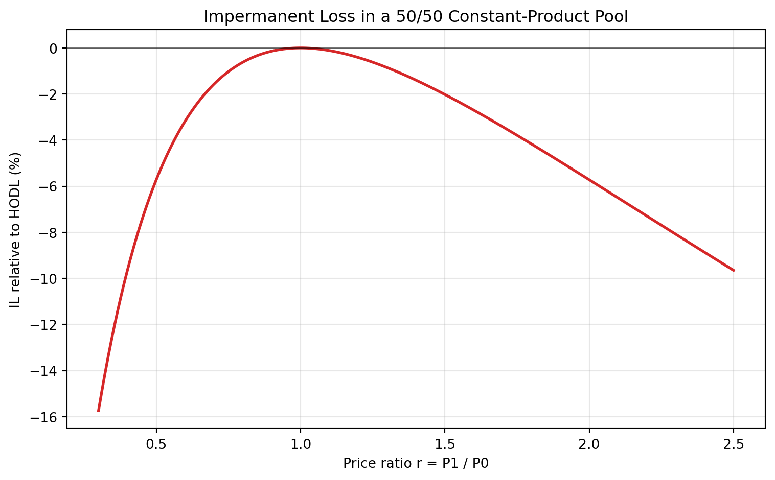
To derive the no-fee IL fraction for a price ratio move from 1 to r=P_1/P_0 in a 50/50 constant-product pool, normalize the initial state to P_0=1 and (x_0,y_0)=(1,1), so k=1. When the external price moves to P_1=r, arbitrage pushes the pool to reserves (x,y) that satisfy
\frac{y}{x}=r,\qquad xy=1,
which implies
x=\frac{1}{\sqrt{r}},\qquad y=\sqrt{r}.
At that point, the LP position is worth (in units of y)
V_{\mathrm{LP}}(r)=y+rx=\sqrt{r}+r\frac{1}{\sqrt{r}}=2\sqrt{r}.
If instead the investor had simply held the initial one unit of each token, the value would be
V_{\mathrm{HODL}}(r)=1+r.
By definition, impermanent loss compares these two values, which gives the result:
\mathrm{IL}(r)=\frac{V_{\mathrm{LP}}(r)}{V_{\mathrm{HODL}}(r)}-1
=\frac{2\sqrt{r}}{1+r}-1.
Because 1+r\ge 2\sqrt{r} by AM-GM, this value is always non-positive, and it becomes more negative as r moves away from 1.
fig, ax = plt.subplots(figsize=(8, 5))ax.plot(r_grid, 100* il, lw=2, color="tab:red")ax.axhline(0, color="black", lw=1, alpha=0.6)ax.set( title="Impermanent Loss in a 50/50 Constant-Product Pool", xlabel="Price ratio r = P1 / P0", ylabel="IL relative to HODL (%)",)ax.grid(alpha=0.3)plt.tight_layout()plt.show()
To break even, fee income must offset IL. A simple approximation is:
\text{LP net return} \approx \text{fee yield} - |\mathrm{IL}|.
So LP profitability depends on the balance between volatility-driven IL and volume-driven fee revenue. DEX transparency helps measure this tradeoff directly, but it does not remove other risks such as smart-contract vulnerabilities and MEV.
# Stylized break-even fee yield for different price movessample_r = np.array([0.7, 0.9, 1.0, 1.1, 1.3, 1.6, 2.0])sample_il =2* np.sqrt(sample_r) / (1+ sample_r) -1show_table(pd.DataFrame({"Price Ratio r = P1 / P0": sample_r,"Impermanent Loss (%)": 100* sample_il,"Break-Even Fee Yield (%)": 100* np.abs(sample_il),}), 3)
Price Ratio r = P1 / P0
Impermanent Loss (%)
Break-Even Fee Yield (%)
0.7
-1.569
1.569
0.9
-0.139
0.139
1.0
0.000
0.000
1.1
-0.113
0.113
1.3
-0.854
0.854
1.6
-2.699
2.699
2.0
-5.719
5.719
How Uniswap v3 and v4 Differ from This Notebook
This notebook uses the v2-style full-range constant-product setup as a baseline. In that baseline, liquidity is active at all prices and the LP share is straightforward.
Uniswap v3 changes this by letting LPs choose an active price range. Fees are earned only while price is in range, so fee income becomes path-dependent:
\text{LP Fee Income}_{1:T}=\sum_{t=1}^{T}s_t\,f_t\,V_t,
where s_t is the LP share of active in-range liquidity. The benefit is higher capital efficiency near current price; the cost is that narrow ranges can go inactive when price moves.
Uniswap v4 keeps concentrated liquidity and adds programmable hooks6 plus a singleton architecture for lower gas costs (Uniswap Labs 2025; Adams et al. 2024). So, relative to this notebook: v3 adds range choice, and v4 adds programmability on top of that.
6 Programmable hooks are optional external contracts attached to a pool that can run at predefined points (for example, before/after swaps or liquidity changes) to implement custom policies such as dynamic fees, order constraints, or specialized accounting rules.
AMMs convert market making into a rule-based reserve system. Constant-product pools are simple and transparent, but they produce endogenous slippage and inventory risk. Arbitrage aligns AMM prices with external markets, yet that alignment changes LP inventory composition.
From a market-structure perspective, DEX AMMs should be viewed less as a brand-new market concept and more as a transparent, programmable version of decentralized currency dealing. They trade off transparency and auditability against a different risk bundle than CEX trading. For empirical analysis, three objects are central: pool depth (price impact), volume (fee income), and volatility (IL pressure). Most LP outcomes can be understood as the interaction of those three forces.