from pathlib import Path
import numpy as np
import pandas as pd

data_dir = Path("../_data")

def load_wrds(name, sql):
    file = data_dir / f"{name}.parquet"
    if not file.exists():
        import wrds
        conn = wrds.Connection()
        df = conn.raw_sql(sql, date_cols=["date"])
        conn.close()
        data_dir.mkdir(exist_ok=True)
        df.to_parquet(file)
    return pd.read_parquet(file)

crsp_m = load_wrds("crsp_msf_1963_2025", """
    SELECT a.permno, a.date, a.ret, a.shrout, a.prc
    FROM crsp.msf AS a
    LEFT JOIN crsp.msenames AS b
      ON a.permno = b.permno
     AND b.namedt <= a.date
     AND a.date <= b.nameendt
    WHERE a.date BETWEEN '1963-01-01' AND '2025-12-31'
      AND b.exchcd BETWEEN 1 AND 3
      AND b.shrcd BETWEEN 10 AND 11
""")

crsp_vw = load_wrds("crsp_msi_1963_2025", """
    SELECT date, vwretd
    FROM crsp.msi
    WHERE date BETWEEN '1963-01-01' AND '2025-12-31'
""")

ff = load_wrds("ff_factors_monthly_1963_2025", """
    SELECT date, rf
    FROM ff.factors_monthly
    WHERE date BETWEEN '1963-01-01' AND '2025-12-31'
""")

ff5 = load_wrds("ff_fivefactors_monthly_1963_2025", """
    SELECT date, mktrf, smb, hml, rmw, cma, umd
    FROM ff.fivefactors_monthly
    WHERE date BETWEEN '1963-01-01' AND '2025-12-31'
""")Implementing the Minimum-Variance Portfolio
The global minimum variance (GMV) portfolio is the one point on the mean-variance frontier of Markowitz (1952) that needs no estimate of expected returns. Every input comes from the covariance matrix.
Markowitz, Harry. 1952. “Portfolio Selection.” Journal of Finance 7 (1): 77–91.
Black, Fischer. 1972. “Capital Market Equilibrium with Restricted Borrowing.” Journal of Business 45 (3): 444–55.
Frazzini, Andrea, and Lasse Heje Pedersen. 2014. “Betting Against Beta.” Journal of Financial Economics 111 (1): 1–25.
The usual way to lower an equity portfolio’s beta is to mix the market with Treasury bills (T-bills), and every such mix has the market’s Sharpe ratio. The GMV portfolio stays fully invested in stocks, holding those whose returns move the least, so it also has a low beta. Under the CAPM it cannot beat the T-bill mix. Black (1972) explains why it might: investors who cannot use leverage buy high-beta stocks to get market exposure, which leaves low-beta stocks with higher returns than the CAPM predicts. Frazzini and Pedersen (2014) document this pattern across asset classes and countries.
Estimating the covariance matrix of 100 stocks from 60 months of returns makes the sample matrix singular, so the textbook GMV portfolio does not exist. Forbidding short sales fixes this, and the resulting portfolio holds only a few stocks.
Each month we take the 100 largest stocks in CRSP with five full years of returns, estimate their covariance matrix from those 60 months, form the long-only GMV portfolio, and hold it for the next month. We compare its returns with the CRSP value-weighted index, a value-weighted portfolio of the same 100 stocks, and a market and T-bill mix with the same beta. We then replace the constraint with shrinkage, vary the number of stocks from 50 to 500, and run factor regressions.
Pulling data from WRDS
Monthly returns, prices and shares outstanding come from crsp.msf, joined to crsp.msenames to keep ordinary common shares (share codes 10 and 11) on the NYSE, AMEX or Nasdaq (exchange codes 1 to 3). The value-weighted market return comes from crsp.msi and the one-month T-bill rate from ff.factors_monthly. The Fama-French five factors and momentum come from ff.fivefactors_monthly. Each table is saved as a parquet file in _data on the first run. Delete a file to pull it again.
Market capitalization, in billions of dollars, uses the absolute price, since CRSP reports the bid-ask midpoint as a negative price when there was no trade. The Fama-French file dates months by their first day and CRSP by the last trading day, so the risk-free rate and the factors are matched by calendar month. With data from January 1963, the first portfolio is held in January 1968. Nasdaq enters CRSP in December 1972, so before then both the universe and the index cover only NYSE and AMEX.
start_date, end_date = "1963-01-01", "2025-12-31"

crsp_m = crsp_m[crsp_m["date"].between(start_date, end_date)].copy()
crsp_m["mcap"] = crsp_m["prc"].abs() * crsp_m["shrout"] / 1e6

rets  = crsp_m.pivot(index="date", columns="permno", values="ret").sort_index()
mcaps = crsp_m.pivot(index="date", columns="permno", values="mcap").reindex(rets.index)
mkt   = crsp_vw.set_index("date")["vwretd"].astype(float)
rf    = ff.set_index(ff["date"].dt.to_period("M"))["rf"].astype(float)
factors = ff5.set_index(ff5["date"].dt.to_period("M")).drop(columns="date").astype(float)
Minimum variance with a singular covariance matrix
With N assets and covariance matrix \Sigma, the GMV portfolio solves
\min_{w} \; w^\top \Sigma w \quad \text{subject to} \quad \sum_{i=1}^N w_i = 1,
with solution w = \Sigma^{-1}\mathbf{1} / (\mathbf{1}^\top \Sigma^{-1} \mathbf{1}). Sixty returns on 100 stocks span at most 59 directions, so the sample matrix assigns zero variance to 41 independent portfolios whatever the true covariances are. This is not noise but missing information: the inverse does not exist, and infinitely many fully invested portfolios have zero sample variance. Shrinkage fills in the missing directions by assumption, and we return to it below.
Forbidding short sales gives
\min_{w} \; w^\top \Sigma w \quad \text{subject to} \quad \sum_{i=1}^N w_i = 1, \quad w_i \geq 0.
The constraint makes no explicit assumption about the missing directions. It rules out the long-short positions that depend on them, so the problem has a solution. It still acts on the estimates implicitly: Jagannathan and Ma (2003) show that it is equivalent to shrinking the largest covariance estimates.
The constraint set is the probability simplex, so we use projected gradient descent: a gradient step on \tfrac{1}{2} w^\top \Sigma w, then an exact sort-based projection onto the simplex. A small ridge term keeps the problem strictly convex, and a step size of 1/L, with L the largest eigenvalue of \Sigma, guarantees convergence.
def proj_simplex(v):
    u = np.sort(v)[::-1]
    cssv = np.cumsum(u)
    rho = np.nonzero(u * np.arange(1, len(v) + 1) > (cssv - 1))[0][-1]
    theta = (cssv[rho] - 1) / (rho + 1)
    w = np.maximum(v - theta, 0.0)
    return w / w.sum()

def minvar_longonly_pgd(S, tol=1e-4, max_iters=10000, ridge=1e-8):
    S = 0.5 * (S + S.T) + ridge * np.eye(S.shape[0])
    n = S.shape[0]
    w = np.full(n, 1 / n)
    eta = 1.0 / np.linalg.eigvalsh(S).max()
    for _ in range(max_iters):
        w_new = proj_simplex(w - eta * (S @ w))
        if np.linalg.norm(w_new - w) < tol:
            return w_new
        w = w_new
    return w
Portfolio formation
At the end of each month t we keep the 100 largest stocks with a return in each of the 60 months ending at t, as Jagannathan and Ma (2003) do, estimate their covariance matrix from that window, and apply the weights to month t+1 returns. Everything is known at t, with one exception: a stock with no return in t+1, typically a delisting, is dropped and the other weights rescaled, which ignores its delisting return.
A value-weighted portfolio of the same stocks separates the effect of the weights from the effect of restricting the universe to large caps. The CRSP index uses the same weighting but covers all stocks and includes delisting returns.
form_portfolios takes a dictionary of weighting rules, each a function of the return window, and records each portfolio’s return along with the number of stocks held, the effective number of holdings 1/\sum_i w_i^2, the largest weight and the gross exposure \sum_i |w_i|, the dollars held long plus short per dollar invested. Gross exposure equals one for a long-only portfolio and 1 + 2s when short positions total s. form_portfolios first drops stocks that never enter the top 100, which only saves time.
def form_portfolios(rets, mcaps, rules, window=60, top_n=100):
    dates = rets.index

    # Only stocks with a return in each of the last `window` months are eligible
    mcaps = mcaps.where(rets.notna().rolling(window).sum() == window)

    # Keep only stocks that are ever in the top_n at a formation date
    keep = set()
    for t in range(window - 1, len(dates) - 1):
        keep |= set(mcaps.loc[dates[t]].dropna().nlargest(top_n).index)
    cols = sorted(keep)
    rets, mcaps = rets[cols], mcaps[cols]

    out = {}
    for t in range(window - 1, len(dates) - 1):
        dt, dt_next = dates[t], dates[t + 1]

        elig = mcaps.loc[dt].dropna().nlargest(top_n).index
        X = rets.iloc[t - window + 1 : t + 1][elig]

        r_next = rets.loc[dt_next, X.columns].dropna()
        if r_next.empty:
            continue
        w_vw = mcaps.loc[dt, r_next.index]
        row = {"vw": (w_vw / w_vw.sum()) @ r_next}

        for name, rule in rules.items():
            w = pd.Series(rule(X), index=X.columns)
            w_next = w.reindex(r_next.index)
            row[name] = (w_next / w_next.sum()) @ r_next
            row[f"{name}_names"] = (w != 0).sum()
            row[f"{name}_neff"] = 1 / (w ** 2).sum()
            row[f"{name}_max_w"] = w.max()
            row[f"{name}_gross"] = w.abs().sum()
        out[dt_next] = row
    return pd.DataFrame(out).T.astype(float)

def gmv_longonly_sample(X):
    return minvar_longonly_pgd(X.cov().to_numpy())

port = form_portfolios(rets, mcaps, {"gmv": gmv_longonly_sample}, top_n=100)
port["mkt"] = mkt.reindex(port.index)
port["rf"]  = rf.reindex(port.index.to_period("M")).to_numpy()
port = port.dropna()
Results
import matplotlib.pyplot as plt
from matplotlib.ticker import LogLocator, NullLocator, StrMethodFormatter

fig, ax = plt.subplots(figsize=(8, 4.5))
series = [("gmv", "GMV, long-only (top 100)", "#2a78d6"),
          ("vw", "Value-weighted (top 100)", "#eb6834"),
          ("mkt", "CRSP value-weighted (all stocks)", "#1baf7a")]
for col, label, color in series:
    ax.plot((1 + port[col]).cumprod(), label=label, color=color, linewidth=2)
ax.set_yscale("log")
ax.yaxis.set_major_locator(LogLocator(base=10, subs=(1, 2, 5)))
ax.yaxis.set_major_formatter(StrMethodFormatter("{x:g}"))
ax.yaxis.set_minor_locator(NullLocator())
ax.set_ylabel("Growth of $1")
ax.grid(axis="y", color="#e5e5e5", linewidth=0.8)
ax.spines[["top", "right"]].set_visible(False)
ax.legend(frameon=False)
plt.tight_layout()
plt.show()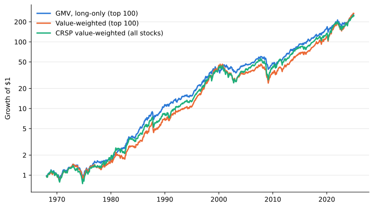
In Table 1 the same-beta mix holds a fraction \beta in the CRSP index and the rest in T-bills, rebalanced monthly, with \beta the full-sample beta of the GMV portfolio. Means and volatilities are annualized. Beta and alpha come from the CAPM regression of excess returns on the market excess return, with two-sided p-values from OLS standard errors.
from scipy.stats import t as t_dist

def summarize(r, m, rf):
    ex, mex = r - rf, m - rf
    X = np.column_stack([np.ones(len(mex)), mex])
    coef, *_ = np.linalg.lstsq(X, ex, rcond=None)
    resid = ex - X @ coef
    se = np.sqrt(resid @ resid / (len(ex) - 2) * np.linalg.inv(X.T @ X)[0, 0])
    wealth = (1 + r).cumprod()
    return pd.Series({
        "Mean (%)": 1200 * r.mean(),
        "Volatility (%)": 100 * np.sqrt(12) * r.std(),
        "Sharpe ratio": np.sqrt(12) * ex.mean() / ex.std(),
        "Beta": coef[1],
        "Alpha (%)": 1200 * coef[0],
        "Alpha p-value": 2 * t_dist.sf(abs(coef[0] / se), len(ex) - 2) if se > 1e-12 else np.nan,
        "Max drawdown (%)": 100 * (wealth / wealth.cummax() - 1).min(),
    })

short = {"gmv": "GMV", "vw": "VW top 100", "mkt": "CRSP VW"}
stats = pd.DataFrame({name: summarize(port[col], port["mkt"], port["rf"]) for col, name in short.items()})
port["mix"] = port["rf"] + stats.loc["Beta", "GMV"] * (port["mkt"] - port["rf"])
stats["Same-beta mix"] = summarize(port["mix"], port["mkt"], port["rf"])
stats.map(lambda x: "" if pd.isna(x) else f"{round(x, 2) + 0.0:.2f}")| GMV | VW top 100 | CRSP VW | Same-beta mix | |
|---|---|---|---|---|
| Mean (%) | 10.48 | 10.98 | 10.95 | 8.38 |
| Volatility (%) | 12.34 | 15.04 | 15.77 | 9.60 |
| Sharpe ratio | 0.49 | 0.44 | 0.41 | 0.41 |
| Beta | 0.61 | 0.92 | 1.00 | 0.61 |
| Alpha (%) | 2.09 | 0.56 | 0.00 | 0.00 |
| Alpha p-value | 0.04 | 0.29 | ||
| Max drawdown (%) | -38.67 | -48.14 | -51.48 | -34.30 |
The GMV portfolio has much lower volatility, beta and drawdown than the market, using only past covariances. The value-weighted top 100 behaves like the market, so the difference comes from the weights, not from the large-cap universe.
The same-beta mix has the same market risk with even lower volatility and drawdown, since the concentrated GMV portfolio also carries idiosyncratic risk. Low beta is what protects both in downturns. The mix has the market’s Sharpe ratio by construction, while the GMV portfolio earns more. The gap in means is the GMV alpha, and it comes from the low-beta tilt, not from a return forecast. Two caveats: the alpha is only borderline significant, with a p-value just below 5%, and the value-weighted top 100 also beats the market’s Sharpe ratio, so part of the gap comes from holding large caps. The factor regressions below ask what the low-beta tilt amounts to.
half = len(port) // 2
rows = ["Mean (%)", "Volatility (%)", "Sharpe ratio", "Beta", "Alpha (%)", "Alpha p-value"]
parts = {}
for sub in (port.iloc[:half], port.iloc[half:]):
    period = f"{sub.index[0]:%b %Y} to {sub.index[-1]:%b %Y}"
    for col, name in short.items():
        parts[(period, name)] = summarize(sub[col], sub["mkt"], sub["rf"])[rows]
sub_stats = pd.DataFrame(parts)
sub_stats.map(lambda x: "" if pd.isna(x) else f"{round(x, 2) + 0.0:.2f}")| Jan 1968 to Jun 1996 | Jul 1996 to Dec 2024 | |||||
|---|---|---|---|---|---|---|
| GMV | VW top 100 | CRSP VW | GMV | VW top 100 | CRSP VW | |
| Mean (%) | 11.78 | 11.01 | 11.62 | 9.18 | 10.95 | 10.27 |
| Volatility (%) | 12.43 | 14.76 | 15.56 | 12.27 | 15.33 | 16.00 |
| Sharpe ratio | 0.41 | 0.29 | 0.32 | 0.57 | 0.57 | 0.51 |
| Beta | 0.66 | 0.92 | 1.00 | 0.56 | 0.92 | 1.00 |
| Alpha (%) | 1.82 | -0.20 | 0.00 | 2.51 | 1.33 | 0.00 |
| Alpha p-value | 0.16 | 0.78 | 0.12 | 0.10 | ||
In Table 2 the GMV portfolio has the lowest volatility and beta in both halves and a positive but individually insignificant alpha. Its Sharpe advantage comes from the first half, which overlaps most of the 1968 to 1999 sample of Jagannathan and Ma (2003), who report a volatility of 12.43% for the long-only minimum variance portfolio of 500 randomly drawn large stocks. In the second half its Sharpe ratio is no higher than that of the value-weighted top 100, even though its alpha is larger than in the first half.
Jagannathan, Ravi, and Tongshu Ma. 2003. “Risk Reduction in Large Portfolios: Why Imposing the Wrong Constraints Helps.” Journal of Finance 58 (4): 1651–83.
fig, (ax1, ax2) = plt.subplots(2, 1, figsize=(8, 5), sharex=True)
ax1.plot(port["gmv_names"], label="Stocks with positive weight", color="#2a78d6", linewidth=2)
ax1.plot(port["gmv_neff"], label="Effective number of holdings", color="#eb6834", linewidth=2)
ax1.set_ylabel("Stocks")
ax1.set_ylim(bottom=0)
ax1.legend(frameon=False, loc="upper left")
ax2.plot(100 * port["gmv_max_w"], color="#1baf7a", linewidth=2)
ax2.set_ylabel("Largest weight (%)")
ax2.set_ylim(bottom=0)
for ax in (ax1, ax2):
    ax.grid(axis="y", color="#e5e5e5", linewidth=0.8)
    ax.spines[["top", "right"]].set_visible(False)
plt.tight_layout()
plt.show()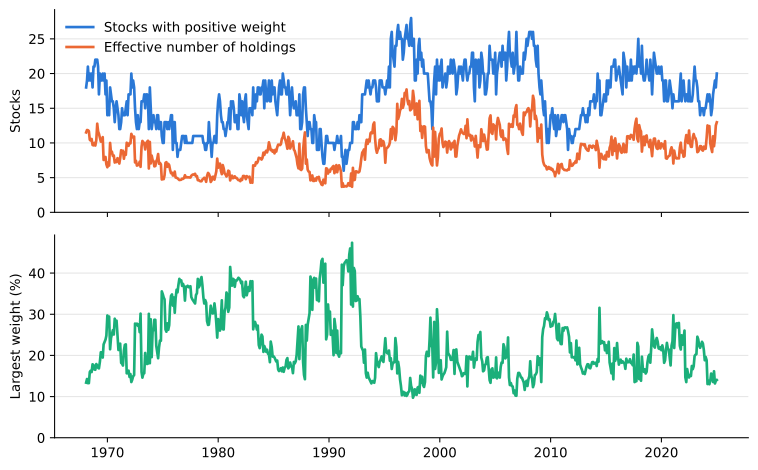
Figure 2 shows the constraint’s second advantage, after making the problem solvable. It binds for most stocks, so the portfolio holds a small subset of the 100, concentrated in names with low volatility and low correlation with the rest. Those names also tend to have low betas, so the GMV portfolio is largely a bet on low beta. Concentration was highest from the 1970s to the early 1990s, eased until 2008, and rose again in 2009 when the financial crisis entered the estimation window.
Shrinking the covariance matrix
Ledoit and Wolf (2004) fill in the missing directions by shrinking the sample matrix S toward a structured target F,
Ledoit, Olivier, and Michael Wolf. 2004. “Honey, i Shrunk the Sample Covariance Matrix.” Journal of Portfolio Management 30 (4): 110–19.
\hat\Sigma = \delta F + (1 - \delta) S, \qquad 0 \leq \delta \leq 1.
Their constant-correlation target keeps each sample variance and sets every correlation to the average \bar r, so F_{ij} = \bar r \, s_i s_j for i \neq j. For any \delta > 0 the blend is invertible and the closed form works again, with the 41 unseen directions governed entirely by the equal-correlation assumption. Their estimate of \delta uses only the window’s returns.
We form the unconstrained GMV portfolio from the closed form and the long-only GMV portfolio from the same solver, both on the shrunk matrix. The first shows what shrinkage does alone, the second whether it adds anything to the constraint.
deltas = {}

def cov_ledoit_wolf(X):
    X = X.to_numpy(dtype=float)
    X = X - X.mean(axis=0)
    T, N = X.shape
    S = X.T @ X / T
    var = np.diag(S)
    s = np.sqrt(var)

    # Constant-correlation target
    r_bar = ((S / np.outer(s, s)).sum() - N) / (N * (N - 1))
    F = r_bar * np.outer(s, s)
    np.fill_diagonal(F, var)

    # Estimated optimal shrinkage intensity
    pi_mat = (X ** 2).T @ (X ** 2) / T - S ** 2
    theta = (X ** 3).T @ X / T - var[:, None] * S
    np.fill_diagonal(theta, 0)
    rho = np.trace(pi_mat) + r_bar * ((s[None, :] / s[:, None]) * theta).sum()
    gamma = ((S - F) ** 2).sum()
    delta = min(1.0, max(0.0, (pi_mat.sum() - rho) / gamma / T))
    return delta * F + (1 - delta) * S, delta

def gmv_unconstrained_lw(X):
    S, deltas[X.index[-1]] = cov_ledoit_wolf(X)
    w = np.linalg.solve(S, np.ones(len(S)))
    return w / w.sum()

def gmv_longonly_lw(X):
    S, _ = cov_ledoit_wolf(X)
    return minvar_longonly_pgd(S)

port_lw = form_portfolios(rets, mcaps, {"lw_un": gmv_unconstrained_lw, "lw_lo": gmv_longonly_lw}, top_n=100)
port = port.join(port_lw.drop(columns="vw"))
delta = pd.Series(deltas)
lw_names = {"gmv": "Long-only, sample", "lw_lo": "Long-only, LW", "lw_un": "Unconstrained, LW"}
lw_stats = pd.DataFrame({name: summarize(port[col], port["mkt"], port["rf"]) for col, name in lw_names.items()})
lw_stats["CRSP VW"] = stats["CRSP VW"]
holdings = pd.DataFrame({name: {"Stocks held": port[f"{col}_names"].mean(),
"Gross exposure": port[f"{col}_gross"].mean()}
for col, name in lw_names.items()})
holdings.loc["Shrinkage intensity"] = [np.nan, delta.mean(), delta.mean()]
pd.concat([lw_stats, holdings]).map(lambda x: "" if pd.isna(x) else f"{round(x, 2) + 0.0:.2f}")| Long-only, sample | Long-only, LW | Unconstrained, LW | CRSP VW | |
|---|---|---|---|---|
| Mean (%) | 10.48 | 10.81 | 10.86 | 10.95 |
| Volatility (%) | 12.34 | 12.16 | 13.17 | 15.77 |
| Sharpe ratio | 0.49 | 0.53 | 0.49 | 0.41 |
| Beta | 0.61 | 0.54 | 0.39 | 1.00 |
| Alpha (%) | 2.09 | 2.85 | 3.87 | 0.00 |
| Alpha p-value | 0.04 | 0.01 | 0.01 | |
| Max drawdown (%) | -38.67 | -37.97 | -39.31 | -51.48 |
| Stocks held | 16.64 | 19.00 | 100.00 | |
| Gross exposure | 1.00 | 1.00 | 2.67 | |
| Shrinkage intensity | 0.65 | 0.65 |
The average shrinkage intensity in Table 3 is well above one half. With fewer months than stocks, the assumption does more of the work than the data.
Table 3 shows that shrinkage makes the textbook portfolio computable but not better. The unconstrained portfolio has the highest volatility of the three and no better Sharpe ratio than the long-only sample portfolio. Its higher alpha comes with a very low beta and a position in every stock, with gross exposure well above one, so its long positions are financed partly by short sales that must be borrowed and rebalanced monthly.
Adding shrinkage to the long-only portfolio barely changes its risk or the number of stocks held, because the constraint already keeps the portfolio away from the missing directions. It does tilt the holdings toward lower-beta stocks, which raises the Sharpe ratio and the alpha. The alphas of all three portfolios have p-values between 1% and 5%, but they come from the same low-beta tilt, so they are one piece of evidence, not three. Both advantages of the constraint survive: it makes no explicit assumption about the missing directions, and it delivers a short list of long positions.
More stocks than months
The difficulty in the first section is a ratio. Demeaning uses up one of the 60 months, so the sample matrix sees at most T - 1 = 59 directions, and its complexity c = N / (T - 1) is about 1.7 with 100 stocks. Varying N shows how the GMV portfolio behaves on either side of c = 1, a question Hellum et al. (2026) study across many asset universes.
Besides the long-only portfolio, we form the unconstrained GMV portfolio with an infinitesimal amount of shrinkage toward the identity matrix, which Hellum et al. (2026) call ridgeless. When N < T - 1 it is the textbook portfolio. When N > T - 1 it is the fully invested portfolio with zero sample variance that has the smallest sum of squared weights, which makes it the closest to equal weights among the infinitely many portfolios the sample considers riskless. Each universe is the N largest stocks with five full years of returns, so a larger N also adds smaller stocks. The value-weighted portfolio of the same stocks tracks that change. With 500 stocks the long-only solver is slow, so this cell takes most of the notebook’s running time.
def gmv_ridgeless(X):
    S = X.cov().to_numpy()
    z = 1e-8 * np.trace(S) / len(S)
    w = np.linalg.solve(S + z * np.eye(len(S)), np.ones(len(S)))
    return w / w.sum()

sizes = [50, 100, 250, 500]
port_n = {n: form_portfolios(rets, mcaps, {"lo": gmv_longonly_sample, "rl": gmv_ridgeless}, top_n=n)
          for n in sizes}
vol_n = pd.DataFrame({n: 100 * np.sqrt(12) * p[["lo", "rl", "vw"]].std() for n, p in port_n.items()}).T
fig, ax = plt.subplots(figsize=(8, 4))
series = [("lo", "GMV, long-only", "#2a78d6"),
("rl", "GMV, ridgeless", "#eb6834"),
("vw", "Value-weighted", "#1baf7a")]
for col, label, color in series:
ax.plot(vol_n.index, vol_n[col], label=label, color=color, linewidth=2, marker="o", markersize=8)
ax.axvline(59, color="#888888", linestyle="--", linewidth=1)
ax.text(62, 1, "$N = T - 1$", color="#555555", va="bottom")
ax.set_xscale("log")
ax.set_xticks(sizes)
ax.xaxis.set_major_formatter(StrMethodFormatter("{x:g}"))
ax.xaxis.set_minor_locator(NullLocator())
ax.set_xlabel("Number of stocks $N$")
ax.set_ylabel("Volatility (%)")
ax.set_ylim(bottom=0)
ax.grid(axis="y", color="#e5e5e5", linewidth=0.8)
ax.spines[["top", "right"]].set_visible(False)
ax.legend(frameon=False)
plt.tight_layout()
plt.show()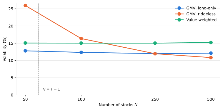
size_stats = {}
for n, p in port_n.items():
    ex = p[["lo", "rl", "vw"]].sub(rf.reindex(p.index.to_period("M")).to_numpy(), axis=0)
    size_stats[f"N = {n}"] = {
        "Complexity N / (T - 1)": n / 59,
        "Volatility, long-only (%)": vol_n.loc[n, "lo"],
        "Volatility, ridgeless (%)": vol_n.loc[n, "rl"],
        "Volatility, value-weighted (%)": vol_n.loc[n, "vw"],
        "Sharpe ratio, long-only": np.sqrt(12) * ex["lo"].mean() / ex["lo"].std(),
        "Sharpe ratio, ridgeless": np.sqrt(12) * ex["rl"].mean() / ex["rl"].std(),
        "Stocks held, long-only": p["lo_names"].mean(),
        "Largest weight, long-only (%)": 100 * p["lo_max_w"].mean(),
        "Gross exposure, ridgeless": p["rl_gross"].mean(),
    }
pd.DataFrame(size_stats).map(lambda x: "" if pd.isna(x) else f"{round(x, 2) + 0.0:.2f}")| N = 50 | N = 100 | N = 250 | N = 500 | |
|---|---|---|---|---|
| Complexity N / (T - 1) | 0.85 | 1.69 | 4.24 | 8.47 |
| Volatility, long-only (%) | 12.80 | 12.34 | 12.00 | 12.12 |
| Volatility, ridgeless (%) | 25.94 | 16.36 | 11.96 | 10.84 |
| Volatility, value-weighted (%) | 15.07 | 15.04 | 15.03 | 15.21 |
| Sharpe ratio, long-only | 0.56 | 0.49 | 0.47 | 0.53 |
| Sharpe ratio, ridgeless | 0.27 | 0.29 | 0.45 | 0.49 |
| Stocks held, long-only | 12.84 | 16.64 | 24.89 | 40.91 |
| Largest weight, long-only (%) | 27.80 | 22.67 | 15.21 | 9.52 |
| Gross exposure, ridgeless | 9.27 | 5.53 | 3.63 | 3.02 |
Figure 3 and Table 4 show two different responses to more stocks. The ridgeless portfolio does worst with 50 stocks, just below c = 1, where the sample matrix is invertible but barely: its volatility exceeds the market’s. Past c = 1 each additional stock adds a direction the sample cannot see, so the set of portfolios with zero sample variance grows and the one closest to equal weights has more room to diversify. Its volatility falls steadily, ending below that of the long-only portfolio with 500 stocks, and its gross exposure falls by about two thirds. This is the pattern Hellum et al. (2026) document: once N exceeds T, more assets help rather than hurt.
Hellum, Oliver, Theis I. Jensen, Bryan T. Kelly, and Semyon Malamud. 2026. Complex Modern Portfolio Theory. Working Paper No. 35246. National Bureau of Economic Research.
The long-only portfolio barely responds. Its volatility is close to the same at every size, because the constraint already keeps it away from the missing directions, and more stocks only spread its weights over more names with a smaller largest weight. It keeps the higher Sharpe ratio at every size. Its Sharpe ratio is highest with 50 stocks, but the differences across sizes are within sampling error. The volatility of the value-weighted portfolio does not change with N, so the change in the universe does not by itself change risk.
Factor exposures
The CAPM alphas measure the gain over the same-beta mix, which is the comparison an investor choosing between the two faces. They do not say whether the GMV portfolios earn anything beyond the premiums of known factors. Table 5 regresses their excess returns on the five factors of Fama and French (2015) and the momentum factor of Carhart (1997).
Fama, Eugene F., and Kenneth R. French. 2015. “A Five-Factor Asset Pricing Model.” Journal of Financial Economics 116 (1): 1–22.
Carhart, Mark M. 1997. “On Persistence in Mutual Fund Performance.” Journal of Finance 52 (1): 57–82.
def factor_regression(r, rf, F):
    ex = (r - rf).to_numpy()
    X = np.column_stack([np.ones(len(ex)), F.to_numpy()])
    coef, *_ = np.linalg.lstsq(X, ex, rcond=None)
    resid = ex - X @ coef
    se = np.sqrt(resid @ resid / (len(ex) - X.shape[1]) * np.diag(np.linalg.inv(X.T @ X)))
    r2 = 1 - resid @ resid / ((ex - ex.mean()) @ (ex - ex.mean()))
    p = 2 * t_dist.sf(np.abs(coef / se), len(ex) - X.shape[1])
    return coef, p, r2

F = factors.reindex(port.index.to_period("M"))
rows = ["CAPM alpha (%)", "CAPM alpha p-value", "Alpha (%)", "Alpha p-value",
        "Market", "SMB", "HML", "RMW", "CMA", "UMD", "R-squared"]
ff_stats = {}
for col, name in {**lw_names, "vw": "VW top 100"}.items():
    capm, capm_p, _ = factor_regression(port[col], port["rf"], F[["mktrf"]])
    coef, p, r2 = factor_regression(port[col], port["rf"], F)
    ff_stats[name] = pd.Series([1200 * capm[0], capm_p[0], 1200 * coef[0], p[0], *coef[1:], r2], index=rows)
pd.DataFrame(ff_stats).map(lambda x: "" if pd.isna(x) else f"{round(x, 2) + 0.0:.2f}")| Long-only, sample | Long-only, LW | Unconstrained, LW | VW top 100 | |
|---|---|---|---|---|
| CAPM alpha (%) | 1.85 | 2.63 | 3.70 | 0.18 |
| CAPM alpha p-value | 0.07 | 0.02 | 0.02 | 0.71 |
| Alpha (%) | -0.41 | 0.16 | 0.36 | 0.00 |
| Alpha p-value | 0.67 | 0.88 | 0.80 | 1.00 |
| Market | 0.72 | 0.67 | 0.56 | 0.98 |
| SMB | -0.23 | -0.25 | -0.32 | -0.27 |
| HML | 0.08 | 0.13 | 0.14 | -0.03 |
| RMW | 0.15 | 0.16 | 0.25 | 0.05 |
| CMA | 0.23 | 0.25 | 0.36 | 0.01 |
| UMD | 0.03 | 0.01 | 0.01 | 0.02 |
| R-squared | 0.70 | 0.62 | 0.40 | 0.98 |
Fama, Eugene F., and Kenneth R. French. 2015. “A Five-Factor Asset Pricing Model.” Journal of Financial Economics 116 (1): 1–22.
Carhart, Mark M. 1997. “On Persistence in Mutual Fund Performance.” Journal of Finance 52 (1): 57–82.
The first two rows repeat the CAPM regression with the Fama-French market factor in place of the CRSP index. The alphas fall a little: that of the long-only sample portfolio is no longer significant, and that of the value-weighted top 100 nearly vanishes. The CRSP index includes securities, such as ADRs and REITs, that the factor excludes, so the significance in Table 1 depends on the choice of market proxy.
Adding the other factors removes every alpha. The GMV portfolios load positively on profitability (RMW) and conservative investment (CMA) and negatively on size (SMB), the pattern Fama and French (2016) find for low-beta and low-volatility stocks, while the momentum loading is close to zero. The alpha attributed above to the low-beta tilt is therefore equally a tilt toward large, profitable firms that invest conservatively. In the data these are largely the same stocks.
Fama, Eugene F., and Kenneth R. French. 2016. “Dissecting Anomalies with a Five-Factor Model.” Review of Financial Studies 29 (1): 69–103.
This does not make the GMV portfolio redundant. The factors are long-short portfolios that include small stocks and are rebalanced on accounting data. The GMV portfolio gets its exposure to the same premiums with a short list of long positions in the 100 largest stocks, chosen from past covariances alone, without any accounting data.
What we learned
With 100 stocks and 60 months, the sample covariance matrix sees only 59 directions, and no computation recovers the rest. Every portfolio in this notebook fills them in with an assumption: the constraint with a sign restriction, Ledoit-Wolf shrinkage with equal correlations, and the ridgeless portfolio with a preference for equal weights. The assumptions differ, but the outcomes mostly agree. The long-only portfolios at every size, the shrinkage portfolios, and the ridgeless portfolio with 250 or more stocks all have volatility 16% to 31% below the market’s. The risk reduction reflects structure in stock returns, not a feature of one estimator. The choice to avoid is the intuitive one: keeping fewer stocks than months so that the inverse exists puts the problem next to c = 1, where the textbook portfolio is riskier than the market.
The versions differ in what an investor has to hold. The long-only portfolio delivers the risk reduction with a short list of long positions, while the unconstrained versions hold every stock in the universe with gross exposure of at least two and a half times capital. The factor regressions show what the returns are: the GMV portfolios earn the premiums of large, profitable firms that invest conservatively, and they find those firms using only past covariances.
The long-only portfolio is still a research portfolio. It holds a few stocks with large weights, trades every month, and its returns are before trading costs. Weight caps, sector limits, slower rebalancing and a factor risk model are the steps toward an investable defensive portfolio.