Performance Evaluation
Investment Theory
Fall 2026
Why Measure Performance?
- Investors hand money to managers in the hope that they know something the market does not.
- Pension funds hire dozens of managers; individuals choose among thousands of funds.
- Each decision needs a comparison of the fund’s record with what the investor could have earned without the manager.
- Questions:
- How do we measure the return?
- How do we adjust it for risk?
- How precise is the answer?
- Where did the return come from?
Time-Weighted and Dollar-Weighted Returns
- The time-weighted return compounds the return of each period:
1 + \bar{r}_{\text{TW}} = \left[ (1 + r_{1}) (1 + r_{2}) \cdots (1 + r_{T}) \right]^{1/T}.
\tag{1}
- It measures what the manager did with each dollar.
- The dollar-weighted return is the internal rate of return of the investor’s cash flows:
C_{0} + \sum_{t = 1}^{T - 1} \frac{C_{t}}{(1 + \bar{r}_{\text{DW}})^{t}} = \frac{V_{T}}{(1 + \bar{r}_{\text{DW}})^{T}}.
\tag{2}
- It measures what investors earned, including how well they timed their purchases.
Example 1 (A Fund with Bad Timing) A fund starts with $100 million, returns 50\% in its first year, attracts $150 million of new money, and returns -20\% in its second year. Its time-weighted return is (1.5 \times 0.8)^{1/2} - 1 = 9.54\% a year. It ends with 0.8 \times 300 = \$240 million, so the dollar-weighted return solves 100 + 150/x = 240/x^{2}, which gives x = 0.9712, or -2.88\% a year. Investors put in $250 million and ended with $240 million.
The ARK Innovation ETF
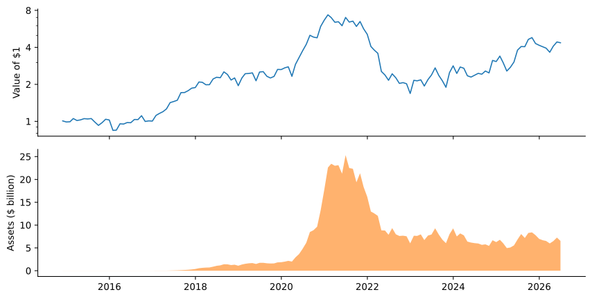
Growth of $1 invested in the ARK Innovation ETF at its launch, on a log scale (top), and the fund’s total net assets in billions of dollars (bottom).
The Manager’s Record and the Investors’
- Time-weighted: the fund compounded at 13.5% a year, November 2014 to June 2026.
- Assets were tiny in its best years and peaked at $25.3 billion in June 2021, just before the collapse of 2022.
- Dollar-weighted: investors as a group earned -5.5% a year.
- Investors put in $10.6 billion more than they took out, and ended $4.1 billion below what they had invested.
- Performance evaluation uses time-weighted returns, net of expenses for investors and gross of expenses to judge the manager.
Adjusting for Risk
- Notation: a fund’s excess return R_{P} has mean \mu_{P}, volatility \sigma_{P}, beta \beta_{P} and residual volatility \sigma(e_{P}); the market has \mu_{M} and \sigma_{M}.
- Sharpe ratio (Sharpe 1966) and M² (Modigliani and Modigliani 1997):
\mathit{SR}_{P} = \frac{\mu_{P}}{\sigma_{P}} \qquad M^{2}_{P} = \frac{\sigma_{M}}{\sigma_{P}} \mu_{P} - \mu_{M} = \sigma_{M} (\mathit{SR}_{P} - \mathit{SR}_{M}).
- M² levers or unlevers the fund to the market’s volatility and compares returns.
- Treynor’s measure (1965) and Jensen’s alpha (1968):
T_{P} = \frac{\mu_{P}}{\beta_{P}} \qquad \alpha_{P} = \mu_{P} - \beta_{P} \mu_{M}.
- T_{P} - \mu_{M} = \alpha_{P} / \beta_{P}, so the two always agree on the sign.
The Information Ratio
- The information ratio scales alpha by the residual risk that comes with it: \mathit{IR}_{P} = \frac{\alpha_{P}}{\sigma(e_{P})}.
- From the Treynor-Black model, combining the fund with the market in the best proportions gives \mathit{SR}^{2} = \mathit{SR}_{M}^{2} + \mathit{IR}_{P}^{2}.
- A large alpha with a lot of residual risk can be used only in small doses.
Which Measure?
| The fund is | Use | Because |
|---|---|---|
| The investor’s whole risky portfolio | Sharpe ratio or M² | All of its volatility is borne |
| One of many funds held together | Treynor’s measure or alpha | Residual risk diversifies away |
| An active portfolio added to an index fund | Information ratio | It sets the gain in the overall Sharpe ratio |
Example 2 (One Fund, Three Verdicts) The market has \mu_{M} = 7\% and \sigma_{M} = 18\%, so \mathit{SR}_{M} = 0.389. A fund has \mu_{P} = 9\%, \sigma_{P} = 25\% and \beta_{P} = 1.2. Then \mathit{SR}_{P} = 0.36 and M^{2}_{P} = 18\% \times (0.36 - 0.389) = -0.52\%, but T_{P} = 7.5\% > 7\% and \alpha_{P} = 9\% - 1.2 \times 7\% = 0.6\%. Its residual volatility is \sqrt{0.25^{2} - 1.2^{2} \times 0.18^{2}} = 12.6\%, so \mathit{IR}_{P} = 0.048. As the only holding, it is worse than the market; as one of many funds, it is better; added to an index fund, it is nearly worthless.
Measures for Real Funds
| Mean | Vol. | Sharpe | M² | Beta | Treynor | Alpha | t | IR | |
|---|---|---|---|---|---|---|---|---|---|
| Vanguard 500 | 10.3 | 15.3 | 0.67 | 0.1 | 0.97 | 10.7 | 0.1 | 0.39 | 0.09 |
| Magellan | 9.5 | 17.9 | 0.53 | -2.2 | 1.08 | 8.8 | -1.9 | -1.52 | -0.35 |
| Contrafund | 12.0 | 15.5 | 0.77 | 1.6 | 0.93 | 12.9 | 2.2 | 1.87 | 0.43 |
| Growth Stock | 11.2 | 17.7 | 0.63 | -0.6 | 1.05 | 10.7 | 0.2 | 0.11 | 0.03 |
| Windsor | 8.4 | 17.1 | 0.49 | -2.8 | 1.02 | 8.2 | -2.3 | -1.76 | -0.40 |
| Dodge & Cox | 8.7 | 17.6 | 0.49 | -2.8 | 1.04 | 8.3 | -2.3 | -1.56 | -0.36 |
| Primecap | 12.5 | 15.9 | 0.78 | 1.8 | 0.96 | 13.0 | 2.4 | 2.10 | 0.48 |
| Sequoia | 7.5 | 16.3 | 0.46 | -3.2 | 0.85 | 8.8 | -1.4 | -0.68 | -0.16 |
| Market | 10.5 | 15.8 | 0.67 | 0.0 | 1.00 | 10.5 |
- Annualized, from net returns, July 2006 to June 2026. Mean, volatility, M², Treynor and alpha in percent.
Reading the Table
- The rankings mostly agree: Primecap and Contrafund top every measure, with Sharpe ratios of 0.78 and 0.77 against 0.67 for the market.
- Diversified funds with betas near one: volatility and beta convey nearly the same information.
- The exception is Sequoia, a concentrated fund with beta 0.85.
- Its Treynor measure ranks it with Magellan, its Sharpe ratio ranks it last.
- The index fund’s alpha of 0.13% is indistinguishable from zero, but its beta is 0.97: the S&P 500 holds large firms only.
Multifactor Alphas
| Alpha | t | MKT | SMB | HML | RMW | CMA | UMD | R^{2} | |
|---|---|---|---|---|---|---|---|---|---|
| Vanguard 500 | -0.33 | -1.83 | 1.00 | -0.12 | 0.03 | 0.05 | 0.02 | -0.00 | 1.00 |
| Magellan | -2.28 | -2.07 | 1.11 | -0.09 | -0.14 | -0.02 | -0.14 | 0.02 | 0.93 |
| Contrafund | 1.08 | 1.25 | 0.98 | -0.09 | -0.15 | 0.07 | -0.18 | 0.09 | 0.94 |
| Growth Stock | -0.17 | -0.18 | 1.07 | -0.06 | -0.29 | -0.06 | -0.27 | 0.01 | 0.95 |
| Windsor | -1.24 | -1.37 | 0.96 | 0.09 | 0.26 | 0.01 | 0.11 | -0.09 | 0.95 |
| Dodge & Cox | -1.29 | -1.28 | 0.98 | 0.01 | 0.31 | 0.04 | 0.09 | -0.11 | 0.94 |
| Primecap | 2.57 | 2.28 | 0.97 | -0.05 | 0.05 | -0.13 | -0.03 | 0.04 | 0.91 |
| Sequoia | -1.14 | -0.53 | 0.81 | 0.14 | 0.05 | 0.12 | -0.15 | -0.02 | 0.69 |
- Growth funds load negatively on HML and CMA; Windsor and Dodge & Cox positively on HML.
- Magellan’s alpha falls to -2.3% (t = -2.07). Primecap is the only fund with a significant positive alpha under both models.
How Precise Is a Measured Alpha?
- Over T years, the standard error of alpha is about \sigma(e_{P}) / \sqrt{T}, so t(\hat{\alpha}_{P}) \approx \frac{\alpha_{P}}{\sigma(e_{P}) / \sqrt{T}} = \mathit{IR}_{P} \sqrt{T}. \tag{3}
- A t of 2 needs T = (2 / \mathit{IR}_{P})^{2} years: 16 for an excellent \mathit{IR} of 0.5, 64 for 0.25.
- Primecap: \mathit{IR} = 0.48 over 20 years gives t \approx 2.15; the regression gives 2.10.
- Sharpe ratios are no more precise (Lo 2002):
\operatorname{SE}(\widehat{\mathit{SR}}) = \sqrt{\frac{1 + \mathit{SR}^{2} / 2}{T}}.
- The market’s 95% interval, 0.23 to 1.11, contains every fund.
Style Analysis
- Sharpe (1992): find the mix of cheap index funds that tracks the fund most closely, \begin{gathered} r_{P,t} = \sum_{j = 1}^{n} w_{j} r_{j,t} + e_{P,t}, \\ \min_{w} \operatorname{V}(e_{P}) \quad \text{subject to} \quad \sum_{j} w_{j} = 1, \quad w_{j} \geq 0. \end{gathered}
- The mix is the fund’s style; the residual is the return due to selection.
- Here the asset classes are four Vanguard index funds (large and small, value and growth) and T-bills.
Style Weights
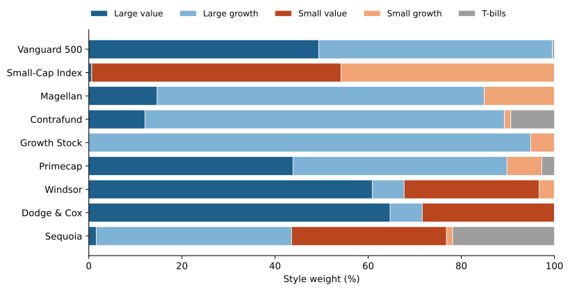
Style weights of seven active funds and two index funds, estimated on monthly returns of four Vanguard index funds and T-bills.
What Style Analysis Shows
- The index funds check the method:
- Vanguard 500: 49% large value, 50% large growth, R-squared 0.998.
- Small-Cap Index: 54% small value, 46% small growth.
- Selection returns, after costs, relative to a passive mix with the same style:
- Primecap 2.4% a year (t = 2.19), Contrafund 1.3% (t = 1.53), Magellan -1.9% (t = -1.84).
- The weights are chosen with hindsight. Sharpe recommended estimating the style from earlier returns only.
Market Timing
- A manager who forecasts the market raises beta before good markets and lowers it before bad ones, making the fund’s return convex in the market’s.
- Treynor and Mazuy (1966): R_{P,t} = \alpha_{P} + \beta_{P} R_{M,t} + \gamma_{P} R_{M,t}^{2} + e_{P,t}.
- Henriksson and Merton (1981):
R_{P,t} = \alpha_{P} + \beta_{P} R_{M,t} + c_{P} \max(-R_{M,t}, 0) + e_{P,t}.
- \max(-R_{M}, 0) is the payoff of a put on the market: a good timer gives investors c_{P} puts for free.
Timing in the Data
- Seven of the eight funds have a negative \gamma_{P}, and none of the positive estimates is significant.
- The typical fund looks like a perverse timer, with more market exposure before low returns.
- Ferson and Schadt (1996): much of this reflects public information.
- Dividend yields and interest rates predict returns, and fund betas move with them for reasons unrelated to skill.
- One mechanism: money flows in when the public expects high returns, and the extra cash lowers beta.
- Conditional measures make perverse timing go away.
- Convexity can also come from holding options, which the manager pays for through a lower alpha.
Performance Attribution
- A sponsor sets a policy weight w_{B,j} for each asset class; the manager deviates through timing and selection (Brinson et al. 1986).
| Index returns | Actual returns | |
|---|---|---|
| Policy weights | I: \sum_{j} w_{B,j} r_{B,j} | III: \sum_{j} w_{B,j} r_{P,j} |
| Actual weights | II: \sum_{j} w_{P,j} r_{B,j} | IV: \sum_{j} w_{P,j} r_{P,j} |
- Timing is II - I, selection is III - I, and the interaction is IV - III - II + I.
Example 3 (Attributing a Balanced Fund’s Return) Policy: 60% stocks, 30% bonds, 10% cash; index returns 8%, 3% and 1%. The fund held 70%, 25% and 5%, and earned 9%, 2.5% and 1% in each class. Then I = 5.8%, II = 6.4%, III = 6.25% and IV = 6.975%. The fund beat its policy by 1.175\%: timing 0.6\%, selection 0.45\% and interaction 0.125\%.
What 93.6% Means
- In 91 large pension plans, 1974 to 1983, the policy explained on average 93.6% of the variation of each plan’s quarterly returns over time.
- It does not say that asset allocation explains 94% of the differences in returns across funds.
- Active management cost the plans about 1.1% a year: 9.01% against 10.11% for their policies.
Benchmarks from Holdings
- Daniel et al. (1997) match each stock a fund holds with one of 125 portfolios formed on size, book-to-market and past return.
- Characteristic selectivity: stock returns minus their matched portfolios.
- Characteristic timing: shifting toward characteristics before they pay off.
- Average style: the return of the fund’s average characteristics.
- Over 2,500 funds, 1975 to 1994: some selectivity, especially in aggressive-growth funds, no characteristic timing, and gains no larger than the extra fees of active funds.
Gaming the Measures
- Goetzmann et al. (2007): changing leverage or trading options, with no information, can raise the Sharpe ratio, alpha and timing measures.
- A measure that cannot be gamed this way must be a certainty equivalent: \hat{\Theta} = \frac{1}{(1 - \rho) \Delta t} \ln \left[ \frac{1}{T} \sum_{t = 1}^{T} \left( \frac{1 + r_{t}}{1 + r_{f,t}} \right)^{1 - \rho} \right].
- Example: monthly returns of -10\%, 5\%, 17\% and -2\% with T-bills at 1% give \hat{\Theta} = 6.6\% with \rho = 2 and 1.2\% with \rho = 3.
- Morningstar’s star ratings use nearly the same measure, with \rho = 3.
Takeaways
- Time-weighted returns judge the manager; dollar-weighted returns describe the investors.
- Sharpe, Treynor, alpha and the information ratio answer different questions.
- Multifactor alphas separate skill from cheap style tilts.
- Alphas and Sharpe ratios are imprecise: decades of data are needed.
- Style analysis, timing regressions and attribution show where a return came from.
- A good measure must be hard to game.